Inside Spacewar!
Part 6: Fatal Attraction — Gravity
(Introduction · The Code · Gravity's End [Scylla] · The Merciless Ship Sucker [Charybdis] · Blazing in the Sun [Pof!] · Excursus – De Computatione Mechanica · Spacewar 4.x and the Hardware Multiply/Divide · A Final Note on Gravity)
In this part of our journey through the internals of Spacewar!, the first digital video game, we're paying another visit to the heavy star. While we've already seen in Part 2 how its flashing presence would have been brought onto the scope, we're now going to investigate how it would unfold its influence on the gameplay by its ever present, all-encompassing effect on the spaceships, the single constant of the Spacewar!-universe and the driving force of space tactics: gravity.
In other words, it's math time in "Inside Spacewar!". But be assured, there's nothing ahead to be afraid of.
It even provides a pretext for some nice graphics like this one:
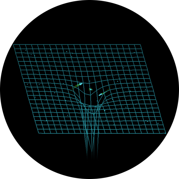
The field of gravity in Spacewar!
(Special purpose emulation with gravity mapping, isometric projection.)
BTW: ▶ You can play here the original code of Spacewar! running in an emulation.
This piece of code, responsible for calculating the effects of the heavy star was done by Dan Edwards, and we also know, how it came into being, thanks to Martin Graetz's seminal article "The Origin of Spacewar" (Creative Computing, 1981) quoting Steve Russell as follows:
Russell: "Dan Edwards was offended by the plain spaceships, and felt that gravity should be introduced. I pleaded innocence of numerical analysis and other things" — in other words, here's the whitewash brush and there's a section of fence — "so Dan put in the gravity calculations."
We've already seen in the previous episode (Part 5) where this piece of code would have been placed — and there's already something interesting about it:
	jda sin		// get sine and store it
	dac \sn
	dzm \bx		// clear \bx and \by (gravity factors)
	dzm \by
	szs 60		// sense switch 6 set?
	jmp bsg		// yes, jump to bsg (no star)

	// heavy star related code here

bsg,	cla		// clean up AC from any leftovers
	sad i \mfu	// ... back to business ...
	clf 6
	lac i mth
	jda cos		// get cosine
(As usual, comments starting with double slashes are mine and not in the original code.)
The interesting thing being, where this "fence" was put up. We could argue that the code related to the star would be starting with the clearing of the variables \bx and \by which will be holding the resulting factors to be added to the movement of the ship, quite like the final check for sense switch 6 (and the conditional jump to label bsg immediately following to this). This, and the clearing of the accumulator (cla) at label bsg is the "fence". But what's on either side of this "section"? The jump to the subroutine for the sine of the turning angle (\mth as in theta) at the one side, and the same for the cosine at the other one. Provided it would be quite "natural" to have them in a common block at either side of the gap, this seems to be a bit like a statement, quite like, "Now, there you are — now, this was really an interruption and here we're back to business, get off my lawn!" Or we could view it rather as some kind of emphasis, like a Sperrung or caesura (the seperation of adjactive and noun in poetry), a framing order, which is emphasizing the separated elements.
However, this rather peculiar placement was kept in each of the various versions of Spacewar!, from the earliest known version, 2b, to the last one, 4.8, despite off any refactoring, even when the code itself was changed for the update of the hardware multiply/divide option in version 4.
Now, let's have a look at this code, as usual, it's Spacewar 3.1, and as usual, we won't do so, without including the standard credits first:
Spacewar! was conceived in 1961 by Martin Graetz, Stephen Russell, and Wayne Wiitanen. It was first realized on the PDP-1 in 1962 by Stephen Russell, Peter Samson, Dan Edwards, and Martin Graetz, together with Alan Kotok, Steve Piner, and Robert A Saunders. Spacewar! is in the public domain, but this credit paragraph must accompany all distributed versions of the program.
The Code
	lac i mx1
	sar 9s
	sar 2s
	dac \t1
	jda imp
	lac \t1
	dac \t2
	lac i my1
	sar 9s
	sar 2s
	dac \t1
	jda imp
	lac \t1
	add \t2
	sub str
	sma i sza-skp
	jmp pof
	add str

	dac \t1
	jda sqt
	sar 9s
	jda mpy
	lac \t1
	scr 2s
	szs i 20		/ switch 2 for light star
	scr 2s
	sza
	jmp bsg
	dio \t1
	lac i mx1
	cma
	jda idv
	lac \t1
	opr
	dac \bx
	lac i my1
	cma
	jda idv
	lac \t1
	opr
	dac \by
(Code as in version 3.1. For the basics of PDP-1 instructions and Macro assembler code, please refer to Part 1.)
As we can see, this is a single strain of code, without a single label, and there are only two jumps to anything outside, one to fast-forward to the label bsg, and one branching to another piece of code at label pof (for point of force or for a more graphical "Poff!"? — however, we learn from the heading comments, what this would be all about):
/ here to handle spaceships dragged into star


/ spaceship in star

pof,	dzm i \mdx
	dzm i \mdy
	szs 50
	jmp po1
	lac (377777
	dac i mx1
	dac i my1
	lac i mb1
	dac \ssn
	count \ssn, .
	jmp srt

po1,	lac (mex 400000	/ now go bang
	dac i ml1
	law i 10
	dac i ma1
	jmp srt
The main part is actually dealing with two different aspects of the star, handling any collisions with it and calculating the influence of gravity, dragging the ships there in the first place. By this Spacewar! is putting its astronauts in the position of a Homeric hero, facing a double monster, while riding their ships through the ether (© E. E. "Doc" Smith) of outer space on the waves of gravity.
Let's start with the first one, the collision detection:
Gravity's End (Scylla)
	lac i mx1	// load x position
	sar 9s		// shift right 11 bits
	sar 2s
	dac \t1		// store it in \t1
	jda imp		// integer multiply AC (x)
	lac \t1		// by \t1 (x)
	dac \t2		// store result in \t2 (x square)
	lac i my1	// load y
	sar 9s		// shift right 11 bits and store it in \t1
	sar 2s
	dac \t1
	jda imp		// integer multiply y (in AC)
	lac \t1		// by y (in \t1)
	add \t2		// add x square
	sub str		// subtract collision radius
	sma i sza-skp	// is it a collision?
	jmp pof		// yes, jump to pof
	add str		// no, add collision radius again (restore sum of squares)
This piece of code is quite straight forward. It starts with loading the x-coordinate of the current objects position (lac i mx1) and shifting it to the right by 11 bits. (We may recall that the maximum amount of positions for a single shift or rotate operation is 9 bits, as in the Macro assembler's constant "9s". Thus, we'll have to split this in two separate instructions, as in "sar 9s" and "sar 2s".) The resulting value in the accumulator is then stored in variable \t1 by the instruction "dac \t1".
So, why would we want to shift this left by 11 bits? We may recall that the positions are stored as screen coordinates in the highest 10 bits (including the sign-bit in bit 0), the lower 8 bits being just fractional values. We're going to perform an integer multiplication on this, therefor we actually have to do some scaling, at least we would want to shift this 8 bits to the right. This is leaving an extra shift by another 3 bits (or division by decimal 8) as the effective scaling. We'll see a bit later, why this would have been applied.
The next two instructions are performing the multiplication. Happens, the PDP-1 doesn't perform any multiplications or divisions out of the box (but there are special instructions for multiply and divide steps performing a dedicated multiple register shift operation). Fortunately, there's BBN (Bolt, Beranek and Newman), and they were friendly enough to supply a multiply subroutine (DEC Memo M-1096, DEC/BBN, 19 Jan 1961), both for single word results and for double precision results:
/BBN multiply subroutine
/Call: lac one factor, jda mpy or imp, lac other factor.

imp,	0		/returns low 17 bits and sign in ac
	dap im1
im1,	xct
	// ... snip ...
	idx im1
	// ... snip ...
	jmp i im1

mpy,	0		/returns 34 bits and 2 signs
	// ... snip ...
According to the heading comment, we're expected to supply one of the two factors in the accumulator and to execute a "jda imp" (for the single precision routine), followed by a "lac" on the other factor, as in "lac \t1". (Actually, a law instruction would do as well, as long as it would be loading the required value into the accumulator.)
How would this work? The instruction jda puts the contents of the accumulator in the memory location specified in the address part and performs a jump to the subroutine in the next address immediately following to this. As with a normal jsr instruction, the current value of the program counter + 1 is put in the accumulator as the return address. By executing "jda imp", we've stored the contents of AC into location imp and are jumping to the next location with the return address in AC. The instruction "dap im1" deposits this in the address part of the location labeled im1, where the opcode xct (execute instruction at given address) is already set up and waiting. This is then executed, and as this instruction happens to be a lac, it will load the second argument into the accumulator. By now, we've the first argument in imp and the second one in AC. In order to jump to a sensible return address, we'll have to finally increment the address in imp and jump there, as in "idx im1" and "jmp i im1".
(We've seen a similar construct in Part 3 and Part 4, where we investigated how the outline compiler would be called.)
For this, the instruction "lac \t1" after the "jda imp" is not overwriting the result of the multiplication (returned in the accumulator), but provides the second factor. The multiply subroutine now returns at "dac \t2", where the result is stored in variable \t2. Thus, the sequence
	dac \t1
	jda imp
	lac \t1
	dac \t2
calculates the square of the value in the accumulator (the modified x-coordinate) and stores the result in \t2.
The next few instructions are repeating this for the y-coordinate in my1. This square of y is then summed with the previously calculated square of x by the instruction "add \t2":
	lac i my1	// load y
	sar 9s		// shift right 11 bits and store it in \t1
	sar 2s
	dac \t1
	jda imp		// integer multiply y (in AC)
	lac \t1		// by y (in \t1)
	add \t2		// add x square
By this, we just computed the square of the distance to the origin of the screen co-ordinates. As luck will have it, this happens to be at the center of the screen, right where the heavy star is placed, liberating us from the task of computing some delta x and delta y values. Thus we are ready to compare this to some epsilon in order to detect a collision. The capture radius (or rather the square of it) is defined in the table of constants at the very top of the source:
str, 15, 1 / star capture radius
This quite lapidar value of 1 is now subtracted from the square and the result (in the accumulator) is then checked for a negative value:
	sub str		// subtract collision radius (1)
	sma i sza-skp	// is it a collision? (not sma or sza)
	jmp pof		// yes, jump to pof
	add str		// no, add collision radius again (restore sum of squares)
The instruction "sma i sza-skp" is a compound instruction that will be performed in a single cycle at once, like we've seen it already in other parts of the source: It sums the instructions sma (skip on minus AC) and sza (skip on zero AC) and subtracts the opcode value of the skip group from this (since this would be represented twice, in each of the two instructions) and the i bit causes the instruction to invert the condition given by this union. (Please mind that the resulting octal instruction 650500 is not the same as "spa" or 640200, the latter simply testing for the sign-bit not being set.) Thus, the next instruction will be skipped, if the accumulator would not be zero or negative (as indicated by a set sign-bit).
If not skipped, the square distance is less then 1 and we have a collision, handled at location pof. — I really love this graphic label! (Someone seems to have been reading Batman or the like.) — Otherwise, we add the value in str again to restore the original value of square distance for later use.
As we may have observed, the capture radius is not that much defined by the constant str, but by the shift to the right by 11 bits. Since a shift to the right by 8 bits would have been perfect for transforming the positional coordinates to integers, we've an extra of 3 bits resulting in a division by 8. Thus, a ship is captured, if the absolute values of both of the coordinates would happen to be less than 8. This would have been quite an expensive calculation for something that could be checked by some simple shifts, if we wouldn't have any other use for the square distance. But if so, we're getting the absolute distance for free to be checked by a single condition. — In fact, we were already deep in the computations of gravity as well:
The Merciless Ship Sucker (Charybdis)
Let there be gravity:
	dac \t1		// store square distance in \t1
	jda sqt		// get the square root of it
	sar 9s		// shift result 9 bits to the right
	jda mpy		// calculate distance x square distance (\t1)
	lac \t1
	scr 2s		// shift result in AC and IO right 2 bits
The instruction "jda sqt" is calling another BBN subroutine, this time for the square root:
/integer square root
/input in ac, binary point to right of bit 17, jda sqt
/answer in ac with binary point between bits 8 and 9
/largest input number = 177777

sqt,	0
	dap sqx
	// ... snip ...
sqx,	jmp .
	// ... snip ...
The heading comment is already providing all we need to know: The first line of the instructions is another (a bit complicated way) of saying that the input is expected to be an integer, the second one is specifying the output format, and we are learning that the highest input processed by this routine is (octal) 177777. (Something we do not learn from this, is where this routine came from. It could be by Adams Associates like the sine-cosine routines, but it's not the same as distributed by DEC in the preliminary memo "M-1092" from 22 Nov. 1960. Or it could be by BBN as well, as suggested by its placement right in between the multiply and the divide subroutines, both by BBN.)
Anyway, we're learning two things here: First, why the positional coordinates were shifted to the right by 11 bits in the first place, and second, why the result is then shifted right by 9 bits. The latter one is easy, since the floating point is right in the middle with 9 bits to the left and 9 bits to the right. This is simply converting the result to an integer.
The first one is mostly related to the maximum input of octal 177777 or decimal 65535: Let's recall, how our input was derived: It's a sum of two squares, which would give us a maximum value for any coordinate of sqrt(65535/2) or (decimal) 181. With our screen postions ranging from -512 to +512, we would have been clearly out of range here and some scaling was needed. Actually, we would have been on the safe side with a shift by two extra bits (making this a maximum of decimal 128), so there's still a single extra shift involved in our initial shift by 11 bits to the right. Let's see ... (While speaking of ranges, the check for a capture radius of less than 1 is preventing us here on performing the square root routine on a zero value, which would probably return an undefined result.)
The resulting square root (now converted to an integer) is then multiplied by the square of the distance (this time calling the double precision 34-bit version of the multiply routine) resulting in the absolute cube of the distance.
This serves also the final solution of the riddle of the initial shift by 11 bits. If we would want to have the value of the resulting cube fitting into a single 18-bit word, we're sailing already hard at the limits with the maximum value of (decimal) 512 scaled to 64, since the cube of 64 is 26,2144, or octal 1000000. Only the absolute values (and some losses by using integer operations only) are preventing an overflow, making this the maximum value for our purpose.
And yet, there's another shift, this time by 2 bits to the rights on the result in the combined AC and IO registers:
scr 2s // shift result in AC and IO right 2 bits
This is obviously scaling the result of the high precision multiply subroutine, but by what amount?
The comment at the call location is providing us with the output format, "returns 34 bits and 2 signs". Seems to be clear enough — but, where would these two signs actually be located? Since the product of two 18-bit words less the sign (making 17 bits) may not exceed 34 bits, this leaves two spare bits. If the signs of the two operands happen to be different, the result is negative and both of the registers are complemented at the end of the procedure (forming a combined 1's complement), making the two spare bits the sign-bits. With the value stretching from AC to IO in consecutive bits, the additional sign-bit is obviously not the highest bit of IO. Where is it located then? Right at the end of IO, by this padding the value by sign-bits at either side. Thus, we've to shift the registers 1 bit to the right in order to make the value in IO an ordinary integer number.
Therefor, this shift by 2 bits is merely resulting in a division by 2.
But we haven't arrived at the end of shifts yet:
	szs i 20	/ switch 2 for light star
	scr 2s
If sense switch 2 would not be zero (mind the i-bit for the inverted condition), we're skipping the next instruction. If zero (not set), we're applying another "scr 2s", thus low gravity will be a quarter of the normal amount. (This might be a bit confusing, but we'll see soon, why a smaller value would effect in a stronger influence of gravity.)
Thus, we just computed a parabolic function as in
(Idealized)  f(x,y) = sqrt((x/8)2 + (y/8)2)3 / 8

Actually:
    x1 = int(x / 8)
    y1 = int(x / 8)
    d2 = x1 * x1 + y1 * y1
    d1 = int(sqrt(d2))
g(x,y) = int((d1 * d2) / 8)

where g(x,y) <= f(x,y)
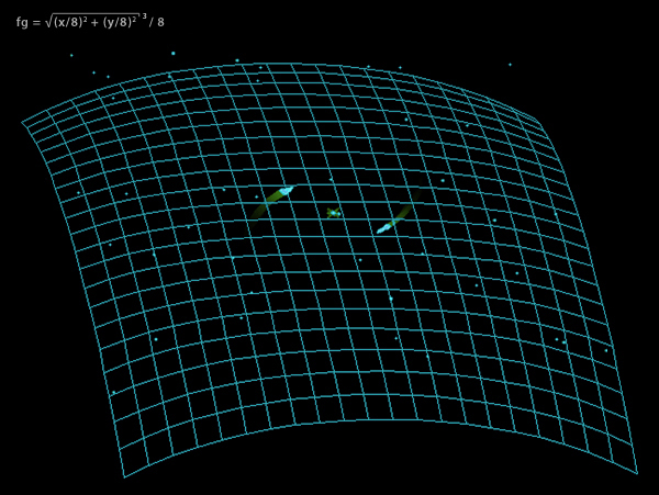
The parabolic function in Spacewar! gravity.
(Isometric projection, orientation of z-axis is downwards.)
The higher part (as in AC) is now checked to be zero. If not, something went utterly wrong and we're aborting the sequence and jump to label bsg, ignoring any gravity for this frame. (This will actually never happen with a regular value, since we shifted the entire result into a single 18 bit value in IO.)
	sza
	jmp bsg
Otherwise, we're calculating the vector of influence, as in \bx and \by (to be added to any other other movement vector in the code following at bsg):
	dio \t1
	lac i mx1
	cma
	jda idv
	lac \t1
	opr
	dac \bx
	lac i my1
	cma
	jda idv
	lac \t1
	opr
	dac \by
First, we're storing the output of our parabolic function in \t1. Since we branched on any non-zero value in the accumulator, this may only be the part left in the IO register, as in "dio \t1". The next instructions are calling the last of the BBN subroutines, the integer divide (DEC Memo M-1097, DEC/BBN, 19 Jan 1961):
/BBN Divide subroutine

/calling squence: lac hi-dividend, lio lo-dividend, jda dvd, lac divisor.
/returns quot in ac, rem in io.

idv,	0		/integer divide, dividend in ac.
	// ... snip ...
dvd,	0
	dap dv1
	// ... snip ...
Once again, we're supposed to provide two factors, the dividend and the divisor. The dividend may be a 36 bit number with the higher part in AC and the lower part in IO (just like the result of the square root routine, maybe a clue for its origin at BBN) for use with the high precision routine dvd or a simple 18 bit value (to be returned in AC) for the low precision routine idv (used here). The divisor is handed over quite like we've already seen it with the multiply routine, by a lac following immediately after the "jda idv". The routine will return at the next instruction in case of an illegal operation as indicated by an overflow, or skip this instruction and return at the next one. For this, the instruction following the "lac \t1" is a simple opr (synonymous to the void instruction nop), providing no handling of this case at all. (We are pretty confident that our code won't end up here.)
Thus, this sequence is loading the x-position (referred to by pointer mx1) into the accumulator and complements this by the following cma instruction. This is then divided by the output of the parablic function in \t1 and the result is stored in variable \bx. (Mind that the value referred to by mx1 is the unshifted x-coordinate, the equivalent of the x-position multiplied by decimal 256.)
The same procedure is then repeated for the y-cordinate in my1 and the result is stored in variable \by.
This is effectively transforming our parabolic function into a vectorized hyperbolic one:
bx(x,y) = -x / f(x/256, y/256)
by(x,y) = -y / f(x/256, y/256)
And since a greater divisor makes for a smaller quotient, we now also understand, why low gravity was achieved by skipping an extra shift to the right.
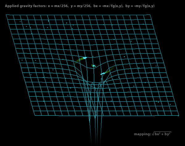
Applied factors of gravity in Spacewar!
(Isometric projection of combined forces along x/y, orientation of z-axis is downwards.)
Let's investigate this a bit more thoroughly, in order to understand it properly. Here is a table of actual inputs and outputs of the gravity calculations for some prominent values of x and y, as calculated for a freely floating spaceship:
Spaceship #1
free falling from 0777/0777 (top right) towards 0/0 (center origin)
all values octal, complete sequence provided for x/y positions < 0100
× ... integer multiply, ÷ ... integer divide, √ ... integer sqrt

f(x,y) = ( √((x >> 3)2 + (y >> 3)2) × ((x >> 3)2 + (y >> 3)2) ) >> 3
\bx = -mx1 ÷ f(mx1 >> 8, my1 >> 8)
\by = -my1 ÷ f(mx1 >> 8, my1 >> 8)

 x      y        mx1      my1      f(x,y)       \bx     \by
777    777     377777   377777     254366         -1      -1
700    700     340177   340177     170760         -1      -1
600    600     300011   300011     113300         -2      -2
500    500     240223   240223      53600         -3      -3
400    400     200000   200000      26400         -5      -5
300    300     140071   140071      11220        -12     -12
201    201     100507   100507       2600        -27     -27
177    177      77726    77726       2235        -33     -33
141    141      60653    60653       1100        -53     -53
120    120      50315    50315        536        -73     -73
101    101      40732    40732        260       -137    -137
 77     77      37612    37612        156       -223    -223
 75     75      36447    36447        156       -216    -216
 72     72      35263    35263        156       -210    -210
 70     70      34056    34056        156       -202    -202
 65     65      32630    32630        110       -276    -276
 62     62      31353    31353        110       -265    -265
 60     60      30047    30047        110       -253    -253
 55     55      26516    26516         53       -415    -415
 52     52      25123    25123         53       -373    -373
 47     47      23471    23471         24       -766    -766
 43     43      21740    21740         24       -713    -713
 40     40      20115    20115         24       -635    -635
 34     34      16207    16207         11      -1453   -1453
 30     30      14133    14133         11      -1264   -1264
 23     23      11731    11731          2      -4754   -4754
 16     16       7031     7031          0          0       0
 10     10       4131     4131          0          0       0
 *capture*
As we may observe, there are some minor discontinuities, due to the limited 18-bit precision, and the result of the divison (\bx = -mx1/f(x,y)) is not decreasing steadily all over the range for mx1, because the intermediate result of the parabolic function f(x,y) not being unique for each value of mx1 and my1. (So, yes, there are actually waves of gravity to ride.) Moreover, the two divisions by zero are yielding a zero result and not some irregular value, while there isn't any handling of this edge-case. (We'll see later why this would be.)
We may also note that while the curvature of this hyperbolic function isn't exactly steep, gravity will be applied at every frame, resulting into a near to immedate plunge into the Star, if we would approach it as near as 34/34 in any direction, unless our ship has an opposing velocity that is compensating or exceeding the pull exerted by gravity. On the other hand, Scylla and Charybdis are not exactly on par and the function will apply the typical sling-shot effect to a ship, if we manage to maneuver closely around the gravitational center in any direction.
Finally, we should note here that, while the gravity factors \bx and \by are directly added to the movement vector in pointers mdx and mdy, only a 2048th part of this vector is applied to a spaceship's postion in each frame. Thus, the most extreme value of 4754 recorded in the series above attributes to an advance of a mere 2 display locations in the same frame, whereas normaly the effect will be building up gradually over a series of frames.
Blazing in the Sun (Pof!)
So, what happens, if our ship falls prey to the Homeric monsters and we happen to collide with the heavy star?
/ here to handle spaceships dragged into star


/ spaceship in star

pof,	dzm i \mdx	// reset x and y
	dzm i \mdy
	szs 50		// sense switch 5 set
	jmp po1		// yes, explode
	lac (377777	// no, reset to antipode
	dac i mx1
	dac i my1
	lac i mb1	// load count of instructions
	dac \ssn
	count \ssn, .	// spend it on counting up in \ssn
	jmp srt		// jump to return of spaceship routine (continues at mb1)

po1,	lac (mex 400000	/ now go bang
	dac i ml1	// store as new control word
	law i 10	// set up explosion timing
	dac i ma1
	jmp srt		// jump to return
As we've seen previously, a square distance smaller than octal 10 will lead to a jump to label pof. Here, the instructions "dzm i \mdx" and "dzm i \mdy" are resetting the x and y velocities of the ship to zero.
What's happening next, is decided on the setting of sense switch 5: If set, we jump to po1 and set up a nice explosion. If not set, the jump is skipped and the spaceship is warped to the antipode by loading 377777 into the two locations in pointers mx1 and my1. "377777" corresponds to the screen location 777/777 (decimal +511/+511) in the upper right corner, where the spaceship will be drawn, split to a quadrant in each of the corners of the screen. But we're not going to display the warping ship (preserving some of the magic), so we'll spend the time involved in a count-up. For this we load the instruction count as stored in pointer mb1 (-4000) into variable \ssn (else used to store the scaled sine) and spend the instruction in an empty loop. When finished, we jump to the exit of the spaceship routine at srt (the jump to the return address, effectively to mb1, just before the end of the comparison loop).
If we end up at label po1, sense switch 5 is set to high for a killing star and we are up to see some pixel dust. As nicely illustrated by the comment, "now go bang", the instruction "lac (mex 400000" is setting up the explosion routine: "mex" is the address of the routine and 400000 is the numerical equivalent of a set sign-bit to indicate a non-colliding state of the ship. This is loaded as a constant expression into the accumulator and deposited as the new control word into the location in pointer ml1 (the handler property of the current object). "law i 10" loads the value -10 to be deposited into the location in pointer ma1, setting up the duration of the explosion. By this, we're done for this frame and jump to the return at srt, happily awaiting the explosion to be displayed in the next frame.
Excursus — De Computatione Mechanica
Cum deus caculat fit mundus. (Leibniz)
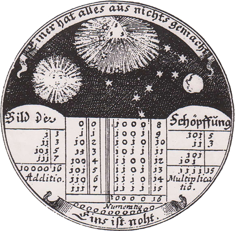
Draft for a medal sent by Leibniz to the duke of Braunschweig-Wolfenbüttel in 1697.
The inscription reads "One has made all from nothing / A one is a nought." (Einer hat alles aus nichts gemacht / Eins ist noht.)
The medal shows an "image of the creation" (Bild der Schöpffung[sic]) as addition and multiplication of binary numbers.
When God calculates, the world arises. If possible, this is even more true for the Spacewar!-universe. But there's a little problem here, since our deus ex machina, arising from the contraption of the PDP-1, isn't exactly good at calculating. Ironically, inspite of its name, a digital computer is good at things like transferring and jamming bits, flipping them, or applying basic Boolean operations to them, but it is exceptionally bad when it comes to computing. A single addition of two binary digits wouldn't be that bad, since it's just an exclusive OR (XOR), but when it comes to numbers, there's a carry involved and we would have to add another XOR, two ANDs, and an inclusive OR, just to perform this on a single digit. Even something as simple as an addition is a serious business involving a serious amount of specialized hardware. Even a binary shift is expensive, but this is an essential operation to any Turing machine, as well as incrementing. It may be or it may be not due to the fact that most humans, if not all, aren't capable of any more complex mathematical operations themselves and are rather resigning to some kind of lookup table of partial results, they've learned to memorize, just like IBM's 1620 (CADET — Can't Add, Doesn't Even Try) did it. But this is not an option for realtime computing.
Multiplication
So, how could we implement something like a multiplication on a binary computer? A naive approach would be a count down on one factor, while adding the other factor to the product in each of the steps. This might be according to the very definition of multiplication, but we would be up for a lengthy procedure involving up to (decimal) 131071 steps for an unsigned 17-bit number. Can't we do any better?
While looking at a binary number, it's obvious that this is representing the sum of 1s multiplied by 2 raised to a power corresponding to a digit's positions. Since multiplication is distributive, it doesn't matter to which of the two factors we would apply this multiplications (or, in terms of electronics, the shifts). Thus, we may just scan one of the factors for 1s and add the other factor to the product with the appropriate number of shifts applied. (Compare Leibniz' medal draft above.)
By this we've arrived at an algorithm that completes in a limited number of steps, one for each digit involved and one operation to be applied, if the scanned number (reduced by shifts itself) would happen to be an odd number. — I believe it was Leibniz, who was quoting Vergil in this context by annotating "numero deus impare gaudet" ("god delights in an odd number"). — Anway, a multiplication step involves a shift on the multiplier to the right to scan the least significant digit, and if we would find this to be what Shakespear called a lucky number, we would add the multiplicant to the product. Since we also need a double length register for a product of two factors of n length, we would rather apply the shift to the product instead of the multiplicant, and add the multiplicant to the higher part.
This is also, what the instruction MUS (multiply step) does. Since the procedure involves both a right shift on the multiplier and a right shift on the double length output register, we may also combine these in a further step of optimization in a single shift: We will start with a cleared accumulator (AC) and one of the factors in IO. Then, for each step, we'll add the other factor (from memory) to the higher part of the double register in AC, if the least significant bit of the combined register would be a 1. Subsequently we'll shift the combined register right by a single bit. In the next step, the next bit of the original multiplier would be in the least significant position and the accumulator would represent a position in the final product relatively shifted left by one bit. If we apply this 17 times (for each unsigned bit), we'll end up with the appropriate result in the combined AC-IO registers. All we have to do is to take care of the signs, since our algorithm is working on unsigned numbers (and ones’ complement representation inverts the individual bits for negative numbers, so that 1s become 0s and vice versa, reversing what’s even what’s odd).
Let's have a look at the full scale multiplication of the BBN subroutine starting at mpy:
/BBN multiply subroutine
/Call. lac one factor, jda mpy or imp, lac other factor.

imp,	0		/returns low 17 bits and sign in ac
	dap im1
im1,	xct
	jda mpy
	lac imp
	idx im1
	rir 1s
	rcr 9s
	rcr 9s
	jmp i im1

mp2,	0

mpy,	0		/returns 34 bits and 2 signs
	dap mp1
	lac mpy
	spa
	cma
	rcr 9s
	rcr 9s
mp1,	xct
	spa
	cma
	dac mp2
	cla
	repeat 21, mus mp2
	dac mp2
	xct mp1
	xor mpy
	sma
	jmp mp3
	lac mp2
	cma
	rcr 9s
	rcr 9s
	cma
	rcr 9s
	rcr 9s
	dac mp2
mp3,	idx mp1
	lac mp2
	jmp i mp1
The jda put's one factor into location mpy and starts at the instruction "dap mp1", complementing its opcode xtc by inserting the address of the instruction that will fetch the other factor. The next instructions are loading the first factor into AC, convert it to an absolute value and swaps them to the IO register. Then the xtc at label mp1 fetchs the other factor in AC and, after converting this one to an absolute value, too, it is stored in mp2. Now, we've one factor in IO and the other in mp2. After the preliminary clearing of AC, we perform the actual multiplication by applying 17 steps of "mus mp2" (as in "repeat 21, mus mp2") — thus computing a raw 34-bit product with the sign-bit in AC and the least significant bit in IO both empty.
Now we're left with the task of appling the appropriate sign. Obviously the product will be negative, when the two factors were of different signs, else the product will be positive. In order to detect the signs, we save AC (the higher value part of the product) in mp2 and once again load the original second factor in AC by "xct mp1" (this will perform another xtc instruction). By performing an exclusive or with the first factor on this and testing for the sign-bit by the instruction sma, we'll either jump to mp3, if the factors were of the same sign, or complement the two parts of the double length product. At mp3 the value in mp1 is incremented to point to the final return address. With the double length registor restored by "lac mp2", we're finsihed and take the jump to the return address.
Notably, the result will be a 34 bit value padded by two signs in AC0 and IO17.
The single length multiplication at imp is a derivative form of this. It will actually execute the routine at mpy that we've just investigated. Then it applies an extra shift in order to normalize the lower part result in IO (for the same reason as we've discussed while inspecting the gravity calculations) and performs a final swap to provide the result in AC.
Division
Division is a bit more complicated. The general algorithm for division is the long division algorithm as in:
Q: quotient, R: remainder, N: dividend, D: divisor

Q := 0
R := 0
for i = n-1..0 do
  R := R << 1
  R(0) := N(i)
  if R >= D then
    R = R - D
    Q(i) := 1
  end
end
Please note that this is using the standard notation with the index starting on the least significant digit, as opposed to the notation used by DEC, numbering the bits from left to right, we're using generally here.
Generally, any division algorithm has to adjust for the following conditions:
dividend = remainder + quotient × divisor, 0 <= remainder < divisor
As we can see, the product of the quotient and the divisor has to be arranged in a way, that it will equal the dividend when summed with a remainder that is less than the divisor. We may see that there is a condition on the remainder for achieving a correct result, and we may see that the only way to arrive at a satisifying value for the remainder is by producing a corresponding quotient (since the divisor is a constant in this procedure). As for the product, we've already seen that we could regard this as a sum of products of powers of two, corresponding to the digits set to one in its factors. We should be able to reverse this procedure, reducing the tasks essentially to exactly knowing where to slice these factors out of the dividend.
We'll start with a partial remainder set to equal the dividend, and like in multiplication, we will scan the number by shifting it one bit at each step. Since this is essentially the reverse operation to multiplication, we'll start at the highest significant digit and shift it to the left (thus dividing it by 2). If the divisor is fitting into the partial remainder (P), as expressed by the condition "P - D >= 0", we'll subtract the divisor (effectively multiplied by 2n-i) and set the corresponding bit in the quotient to high (since the divisor would fit into the dividend for the according times of this power of two).
Thus, we have arrived at the slow division method, generally expressed in:
Pi+1 = R × Pi - qn-(i+1) × D
Or, expressed as an algorithm:
P := N
D := D << n            -- divisor will be implicitly shifted right by n bits
for i = n-1..0 do
  P := 2P - D          -- trial subtraction from shifted value
  if P >= 0 then
    q(i) := 1          -- result-bit 1
  else
    q(i) := 0          -- result-bit 0
    P := P + D         -- new partial remainder is (restored) shifted value
  end
end
Since the subtraction has to be applied to the partial remainder only, if this subtraction is yielding a positive result, we're dealing effectively with two states of the partial remainder, before and after the subtraction, with the condition on the second one. One way to handle this is a non-destructive algorithm, where we would apply the subtraction anyway and restore the partial remainder by adding the divisor again, if the result would be negative (see above). On the other hand, the sign of the partial remainder would indicate the condition for the previous step, so we could put our emphasis on this. If the sign-bit would be unset, the subtraction would have satisfied our condition and we would set the corresponding bit in the quotient. Else, we would add the quotient multiplied by two (to compensate the shift). In both cases, we would then subtract the divisor again, to provide the sign-bit for the next step. Simplifying this, we will either subtract the divisor, if the partial remainder is positive, or we will add the divisor, if it happens to be negative.
For our implementation, we're combining AC and IO into a double-length register once again (since the dividend is a double-length product) and use this for the partial remainder, being initially the dividend. Since we can provide for the corresponding bit position in the quotient by just setting the least significant bit and shifting the quotient to the left as well, we may reuse the AC-IO double-length register and gradually shift in the quotient at the lower side, while the partial remainder is shifted out at the other side. This way, the least significant bit of the double-length register is set to one, if the sign-bit before the shift was unset (indicating a positive partial remainder), and cleared, if the sign-bit is set. In other words, the complemented previous sign-bit becomes the new least significant bit in the gradually produced quotient.
A thing to consider is the sign of the least significant bit shifted in when we would apply the addition for the previous partial remainder being negative. Since the less significant bits in IO will always be positive and the partial remainder is in this case negative (represented in 1's complement), we'll have to add 1 to the addition in order to correct this new bit to the sign. Thus, the addition step becomes "add divisor plus 1", if the sign-bit was negative.
Since each of the steps is presupposing a subtraction previously applied, we'll have to provide for an initial one before applying the first step. Similarly, the last step will apply a surplus one and we'll have to componsate this by a final addition. Moreover, we're dealing with operands of different word length, so we'll have to decide what they would represent. Generally, for this algorithm, they are regarded to represent fractional values, so we will apply the divison to the higher part of the double-length AC-IO register, leaving the part where the quotient is gradually produced intact. (Also, any subtractions or additions will be applied to AC exclusively and we will do fine with any adder-circuitry provided for AC only.) If we would want to use this for an integer divide, we'll have to provide a single-word dividend adjusted to the right of the double-word register in IO only (shifted left one bit to for the sign).
Thus, we've finally arrived at the following algorithm:
0 <= N < 1,  0 < D < 1,  nP = 2nD

D := D << nD           -- D is applied do the higher part of double word P only
P := N

P := P - D             -- initial subtraction
for i = 0..nD-1 do
  s := sign(P)
  P := P << 1
  if is_set(s) then    -- was negative (Pi-1 - D < 0)
    P(lsb) := 0
    P := P + D + 1*    -- *) PDP-1: + 1 corrects 1's complement of AC(lsb) shifted in
  else                 -- was positive (Pi-1 - D >= 0)
    P(lsb) := 1
    P := P - D
  end
end
P := P + D             -- compensate the surplus subtraction applied in last step
The divide step as in instruction DIS expects the dividend in the combined AC and IO registers, and the divisor in the memory location referred to in the address part. At each step the combined registers are shifted left and the complement of the former sign-bit (in AC) is jammed into the least significant position (in IO). If this bit (now in IO bit 17) happens to be 1, the divisor (from memory) is subtracted from AC, else AC is incremented by 1 and the divisor is added. (Actually, the subtraction is performed by an addition, too, complementing AC previously and afterwards.) Applied for each binary digit, it will produce the remainder in AC and will shift the intermediary quotient into IO.
There are actually some constraints on this algorithm: First, it works on absolute values, so we'll have to manage the signs once again on our own. Second, it works only, if the divisor (notably shifted left by a word-length) is greater than the dividend. So, we have an error condition here (an overflow) that is also covering the edge-case of a divsion by zero.
The BBN subroutine is testing the overflow condition after the initial subtraction. If there is an overflow (as indicated by a positive result), the routine returns at the location after the lac for the divisor. If the routine produces a valid result, this instruction is skipped and the routine will return at the next location. Further, there are two entry points: One for a simple integer divide and one for two fractional values with a double-length dividend. The call at dvd is performing a fractional divide (with the fractional point immediately after the sign-bit), the call at idv (as used in Spacewar!) an integer divide on a simple value in AC:
/BBN Divide subroutine

/calling squence. lac hi-dividend, lio lo-dividend, jda dvd, lac divisor.
/returns quot in ac, rem in io.

idv,	0		/integer divide, dividend in ac.
	dap dv1		// store address to fetch the divisor
	lac idv		// load the dividend
	scr 9s		// prepare the dividend: swap it in IO
	scr 8s		//                      (less sign-bit)
	dac dvd		// deposit sign (-0/+0) in dvd
	jmp dv1		// now continue with fractional divide

dvd,	0		// fractional divide
	dap dv1		// store address to fetch the divisor
dv1,	xct		// fetch divisor (in AC)
	spa		// make it an absolute value
	cma
	dac idv		// store divisor in idv
	lac dvd		// load hi-dividend into AC
	sma		// make dividend an absolute value
	jmp dv2
	cma
	rcr 9s
	rcr 9s
	cma
	rcr 9s
	rcr 9s
dv2,	sub idv		// initial subtraction (dividend - divisor)
	sma		// negative? (divisor > dividend)
	jmp dve		// no, abort on overflow
	repeat 22, dis idv	// apply division steps
	add idv		// final addition (compensate surplus subtraction)
	dio idv		// store quotient in idv
	cli		// now arrange sign, first clear IO
	rcr 1s		// rotate AC and IO right 1 bit (sign AC = 0)
	lio dvd		// remainder is same sign as divdend, load hi-dividend
	spi		// dividend was positive?
	cma		// no, complement remainder
	dac dvd		// deposit remainder in dvd
	xct dv1		// compute sign of quotient, fetch divisor
	xor dvd		// xor remainder (get sign diff)
	rcr 9s		// swap AC and IO (store computed sign in IO)
	rcr 9s
	idx dv1		// good divide, increment return address
dve,	idx dv1		// increment return address
	lac idv		// load quotient into AC, arrange sign
	spi		// check sign in IO
	cma		// negative, complement AC (quotient)
	lio dvd		// remainder in IO
	jmp i dv1	// return
The instructions after the final addition are preparing the sign-bits: The remainder is of the same sign as the dividend and the quotient will be negative, if the signs of the divisor and the dividend (or the remainder) are different.
Notably, the input format for the long dividend to be provided for routine dvd is the same as the output format of the high precision multiply routine, a continuous number stretching from AC to IO with no sign in the highest bit of IO. Therefore, if we would want to assemble this from two ordinary values, we would have to apply a shift to the left by one bit position to the low dividend in IO in advance, just like we see it in the preliminary steps of the integer divide routine at idv.
(It is only here that we can see, why the series of Spacewar! gravity factors didn't produce any irregular value on a division by zero and returned 0 instead: Since idv was called for the single-word integer division, AC would have been zero (with the absolute dividend in IO), when the initial subtraction was applied. With zero also subtracted as the divsior, the routine aborted on a positive value by a jump to dve. At this time there's still the divisor in idv, which is now loaded as the result and adjusted to the sign of the absolute dividend, still in IO. Here, this is a small value with the higher bits cleared, resulting in an empty sign-bit. Thus the result returned in AC is a plain zero.)
The automatic hardware multiply/divide option, required by Spacewar! 4.x, is essentially an automatization of these algrorithms performed by the BBN-subroutines with all values generally regarded to represent fractional values. When installed, the instructions multiply step MUS and divide step DIS are replaced by the instructions MUL and DIV respectively (reusing the opcodes of the former single-step instructions). The hardware solution will not only provide the results in fewer cycles, but it will also restore the values in AC and IO, in case a division would return with an overflow.
*****
There is a rather small chance that you, dear reader, would now be asking breathlessly, "And how could we do square roots?" O.k., this may be unlikely, but there are two other, higher order arithmetic subroutines in Spacewar!, namely the square root routine and the sine-cosine routine. And we really should have a look at them, too. Maybe, you, like me, weren't taught a square root algorithm in school, since there had already been this small shiny box, called an electronic calculator (they don't make them shiny anymore), and maybe you are interested in how it came up with its answers. Here is, how it would have done a square root — at least, if it would have been restricted to integer square roots:
*****
Square Roots
When it comes to integer square roots, there is again an approach both naive and literal to the definition: We would go over all the squares of the integers until we would encounter a square that would be greater than our argument. The answer would be the last square before this one, the one that just fitted into the given number. (Since we are dealing here with integers only, we would forget about any remainder.) Again, this is not a viable option for realtime computing and we may want to think about something different. Maybe something that would be working on factors. — But, are there any factors in squares?
We may want to consider the well known formula for solving the square of a binomial term here:
(a + b)2 = a2 + 2ab + b2
From this follows that the square of any number in a number system of base N may be cosidered to be the square of the sum of the various powers of n in this number, as for any 2-digit number x:
x = Np + q
x2  =  (Np + q)2  =  N2p2 + 2Npq + q2
p.e.
95 = 10×9 + 5
952  =  (10×9 + 5)2  =  100×81 + 20×9×5 + 25  =  8100 + 900 + 25  =  9025
If we would want to reverse this, we are learning from the expressions "N2p2" and "q2" (as in "100×81 + 25") that the square parts of this term won't overlap for any two adjacent digits of the root, since the product of any two single-digit numbers must be less than N2 (e.g, (N-1) × (N-1) = 9 × 9 < 100). Thus we may want to scan the square in pairs of two adjacent digits in order to extract the squares of the individual digits of the underlying root. Also, as in division, we will try to extract the biggest factors first, so we will scan the square number from left to right, "bringing off by two".
But there might be some remainder involved and there will be some overlap as in the expression "2Npq". How would we handle this?
Let's see: Considering our base 10 example from above, we inspect the first pair 90, and obviously the biggest square fitting into this is 92. So, we note 9 as the highest digit of our result and subtract its square 81 from 90, makes 9. As we advance to the next digit, bringing down 25 to get q, what does this remainder represent with respect to the square of a binomial?
Substituting N by 10, we get:
x2  =  100p2 + 20pq + q2
q(20p + q)  =  x2 - 100p2

     x2 - 100p2
q = –––––––––––
      20p + q
Generally, the steps we have to apply here are not that much different from solving the remainder and bringing down the next digit in long division, while a bit more complex: Bringing down two involves a shift by two digits to the left (×100), so "x2 - 100p2" represents the remainder of our subtraction, now to be shifted left two digits and the next two digits of the argument added to it. (The other way round, "x2" is the square number as far as we inspected it, and we've already factored out the square of the first root digit(s). As we arrive at q, we have applied a double shift to it and brought down the next two digits, providing the two new lower digits in this for x2 and 100p2, or N2p2.)
In order to get q, we will have to arrange for the divisor in the expression: We will double the partial root, we've just determined, shift it left one digit and add q to it. — Here, we're facing a little problem, since we can't know q at this time. We'll have to come up with a guess.
In our example the dividend is "9×100+25" (or 925) and we have to come up with a guess fo the divisor as in "20×9 + q" (or "180 + q"). In this case we're lucky, since this will work out perfectly with "q = 5", providing the final result 95.
But odds are, we will not be that lucky each time and there will be a remainder. Actually we have to go back and prove our guess:
r = x2 - 100p2 - q(20p + q)
In case we would get a negative remainder, we would have to track back and redo with a smaller guess for q before we would be able to continue with the next pair of digits by bringin down the next two highest digits of the argument at the right of r and q now becoming the next p. — Notably, it is this need for a trial-and-error operation and some potential backtracking which is contributing to the image of this long form method of being rather some kind of dark art or alchemy than an enlightened, clean algorithm.
But see what's happening, when we do the same with binary numbers, with just a single case to be considered, namely q equalling 1:
     x2 - 4p2
q = ––––––––––
      4p + 1

r = x2 - 4p2 - 1(4p + 1)
Amazingly, there is no need for guesses and backtracking with binary numbers: Since q is either 1 or 0, the divisor will either fit into the remainder or not. The term "+ q" becomes a constant expression and the divisor is to be directly solved. With the various multiplications by 4 being the equivalent of double shifts, we arrive at a straight forward algorithm using only basic operations like shifts, increments, and maybe a subtraction:
- Shift any remainder 2 bits to the left, shift in next two highest digits from the argument;
Shift the partial result (p) 1 bit to the left (advance to next digit). - Optional shortcut: Is there any remainder? If zero, continue with step 1 (q = 0).
- Get the divisor by "
(p << 1) + 1" (we already applied one shift to the partial result above) - Does this fit into the remainder?
- If it fits, subtract the divisor from the remainder and increment the partial result by
1(add q). - Repeat for any remaining digits.
Let's have a look at the implementation used by Spacewar!:
/integer square root
/input in ac, binary point to right of bit 17, jda sqt
/answer in ac with binary point between bits 8 and 9
/largest input number = 177777

sqt,	0
	dap sqx		// deposit return address
	law i 23	// load 23 (number of digits to produce + 1)
	dac sq1		// store it in sq1 (loop counter)
	dzm sq2		// clear sq2 (result)
	lio sqt		// load argument into IO
	dzm sqt		// clear sqt, now used for remainder

sq3,	isp sq1		// index sq1, skip on positive (performs 18 iterations)
	jmp .+3		// jump to loop body
	lac sq2		// load sq2 into AC (result)
sqx,	jmp .		// return

	lac sq2		// load partial result
	sal 1s		// shift left 1 bit
	dac sq2		// and store it (sq2 = sq2 << 1)
	lac sqt		// load remainder
	rcl 2s		// combined rotation, multiply & get next 2 bits from IO
	sza i		// is it zero?
	jmp sq3		// yes, continue with next 2 digits at sq3 (root digit is 0)
	dac sqt		// store remainder
	lac sq2		// prepare divisor: load sq2 (partial result)
	sal 1s		// shift left 1 bit
	add (1		// add 1 to it  (ac = sq2 << 1 + 1)
	sub sqt		// subtract remainder (ac ≤ sqt ?)
	sma+sza-skip	// is it zero or minus?
	jmp sq3		// no, continue with next 2 digits (root digit is 0)
	spa		// is it positive?
	cma		// no, complement it
	dac sqt		// store as remainder
	idx sq2		// increment partial result (root digit is 1)
	jmp sq3		// continue

sq1,	0
sq2,	0
Transforming this into some kind of C-like pseudocode (which happens to be valid JavaScript) we get:
function sqrt(num) {
   var result = 0;
   var remainder = 0;
   var divisor, i, t;

   for (i = 0; i < 18; i++) {               // for each resulting digit
      result <<= 1;
      t = (remainder << 2) + (num >> 16);   // this and next line: lac sqt, rcl 2s
      num <<= 2;
      if (t) {
         remainder = t;
         divisor = (result << 1) + 1;
         if (divisor <= remainder) {
            remainder -= divisor;
            result++;
         }
      }
   }
   return result;
}
This is the perfect image of the algorithm we've drafted above: Inside the loop, we first advance to the next digit of our result by applying a shift. Then we apply the double shift to the remainder and add the next two digits to be inspected to it by rotating the combined AC & IO registers, containing the remainder and the argument respectively. If the remainer would now be empty, there's nothing to fit and this digit of the root is a zero. Thus, we may continue by a jump to the next iteration of the loop. (In the assembler code, we won't even store the remainder in this case, since it must have been zero before.) If we've got some remainder, we will check the divisor to fit into the remainder. (This is done by a subtraction and testing the result for being either zero or a negative number. If the divisor fits, it is restored by complementing it.) In case the divisor is less than or equal to the remainder, our result digit is a 1 and we subtract the divisor from the remainder. After repeating this procedure for each bit of our 18-bit result, we're eventually done and return the result.
(Those more familar with the conventional high-school method may want to have a look at the excellent description at http://www.embedded.com/electronics-blogs/programmer-s-toolbox/4219659/Integer-Square-Roots, which is arriving at the very same algorithm.)
What's interesting here on a more textual level, is the clarity of the design of this square routine and its organization in three distinctive blocks, each representing a functional context: The first one at label sqt is storing the return address and initializing the various registers and memory locations used. (We may note the reuse of sqt for the remainder, after the argument, put there by the calling jda instruction, has been transferred to the IO register.) The second one constructs the loop by a single isp instruction (index and skip on positive) that is incrementing the counter and either performs a jump to the loop body, if the contents of the counter would be still negative after the increment, or skips this jump, when the counter becomes zero, and puts the result into the accumulator before jumping to the return address. The main part being the loop body is doing the heavy work, with any branches for another iteration jumping to the loop instruction at label sq3. Finally, there are the two memory registers used for the loop counter and the partial result.
Sine & Cosine
It may be surprising, but there is no standard method to calculate sine and cosine. Moreover, we may not hope to come up with some easy to operate algorithm based on shifts and additions only, since sine and cosine are essentially about projecting a 2D unit vector onto a 1D length. Hence, we may expect to see some higher order functions involved.
While various algorithms are used in computer implementations, like the CORDIC algorithm, then just recently presented in 1959, or the approximation series published in "Approximations for Digital Computers" by Cecil Hastings Jr (Princeton, New Jersey, Princton University Press, 1955, p.138-140) which was also popular at DEC, the sine-cosine routine by Adams Associates, Inc (DEC Preliminary Memo M-1094, 22 Nov 1960) is using the well known Taylor series for approximation:
              x3    x5    x7
sin(x) = x - ––– + ––– - ––– ...
              3!    5!    7!
While this series is actually extending infinitely, we may observe that the higher order terms, like "x9/9!", are becoming smaller and smaller, especially with a small value for x. E.g., for x = 0.1 the 9th order term becomes 0.000000001/362880, a value hardly representable in standard precision. Hence, we may keep the error small and restrict the approximation to just a few terms, as long as we're keeping our arguments small.
Since the sine is both periodical (sin(θ) = sin(θ + 2π)) and symmetrical (sin(θ) = sin(π/2 – θ)), we may reduce the argument to a quadrant (or π/2 radians) in order to keep the error small and to optimize the approximation. And since there is also a symmetry between sine and cosine (a phase shift by π/2), we may use the same core algorithm to approximate both of these functions.
By extracting the constants and rearranging the formula to determine the higher powers of x by repetitive multiplications (Horner scheme), we finally arrive at something that may be implemented on a digital computer:
x = θ/2π   // -1 ≤ x ≤ 1

               (2πx)3   (2πx)5   (2πx)7
sin(x) = 2πx - –––––– + –––––– - ––––––
                 3!       5!      7!

       = C1x + C3x3 + C5x5 + C7x7

       = ((((C7)x2 + C5)x2 + C3)x2 + C1)x
Let's have a closer look at the sine-cosine routine used by Spacewar!. It is actually not the original form of the Adams Associates routine as provided in the Preliminary Memo M-1094 from November 1960, but a revised version, reformatted for use with the Macro assembler and the BBN multiply routine:
/sine-cosine subroutine. Adams associates
/calling sequence= number in AC, jda sin or jda cos.
/argument is between ±2 pi, with binary point to right of bit 3.
/answer has binary point to right of bit 0.  Time = 2.35 ms.

define	mult Z		// macro to call to the BBN multiply routine
	jda mpy		// 34 bit routine
	lac Z
	term

cos,	0		// entrance to cosine, argument deposited here by jda
	dap csx		// routine starts here, deposit return address
	lac (62210	// load π/2
	add cos		// add operand to it
	dac sin		// store in sine
	jmp .+4		// jump to main calculations: cos(x) = sin(π/2+x)

sin,	0		// entrance to sine, argument deposited here by jda
	dap csx		// routine starts here, deposit return address
	lac sin		// load operand
	spa		// is it positive?
si1,	add (311040	// no, add 2π
	sub (62210	// subtract π/2
	sma		// is it minus? (operand was < π/2)
	jmp si2		// no, jump to si2 (reduce)
	add (62210	// restore it (add π/2 again)
			// operand is now -π/2 ≤ AC ≤ π/2, 3 integer bits
si3,	ral 2s		// rotate left 2 bits (now 1 integer bit)
	mult (242763	// × 2/π (with binary point right of sign)
	dac sin		// store x
	mult sin	// get square
	dac cos		// store x^2
	mult (756103	// C7x^2
	add (121312	// C7x^2 + C5
	mult cos	// C7x^4 + C5x^2
	add (532511	// C7x^4 + C7x^2 + C3
	mult cos	// C7x^6 + C5x^4 + C3x^2
	add (144417	// C7x^6 + C5x^4 + C3x^2 + C1
	mult sin	// C7x^7 + C5x^5 + C3x^3 + C1x
	scl 3s		// shift AC & IO left 3 bits (×8)
	dac cos		// store result in cos
	xor sin		// now adjust signs, xor x
	sma		// is it negative? (are result and x of different signs?)
	jmp csx-1	// no, return result (cos)
	lac (377777	// max positive value (2^17-1, nearly 1.0)
	lio sin		// load x into IO
	spi		// is x positive?
	cma		// no, complement AC (400000, 1.0 with bit-shift)
	jmp csx		// jump to return

	lac cos		// load result from cos (as before xor-ing with sin)
csx,	jmp .		// return

si2,	cma		// (operand - π/2 ≥ 0) complement AC
	add (62210	// add π/2
	sma		// is it negative?  (π/2 - opsi2 < 0?)
	jmp si3		// no, jump to main calculations
	add (62210	// add π/2 once more
	spa		// is it positive? (π - opsi2 > 0?)
	jmp .+3		// no, skip next two instructions
	sub (62210	// undo last addition (subtract π/2 again)
	jmp si3		// jump to main calculations

	sub (62210	// subtract π/2 (effectively: ac = π/2 - opsi2)
	jmp si1		// and start over at si1
Our interpretation of the constant values here is backed by the labels in the original code as in Memo M-1094, where "xOy" means x/y and "P" is for π:
	C7	756103
	C5	121312
	C3	532511
	C1	144417
	2OP	242763
	2P	311040
	PO2	062210
	ONE	377777
(To identify the constants otherwise, we have to inspect the binary representation of these fractional octal numbers for equivalents. E.g., "242763" is 010100010111110011 with the binary point just after the sign-bit as in "0.10100010111110011", the equivalent of 2/π or "0.1010001011111001100000110…". Notably, the outer parts at labels si1 and si2 are using a representation with a sign and 3 integer digits, hence "311040" is "0110.01001000100000" or 2π.)
So, what's happening here? Let's start at the sine routine (since the cosine ist quite trivial by adding π/2 to the argument and then continuing with the code for the sine):
The routine is called by "jda sin", hence the argument (or operand) is stored at label sin and the execution starts at the next instruction with the return address in AC. After storing the return address in the address part of location csx the operand is first reduced to the range 0..2π due to the periodicy of the sine. Then, if the operand isn't in the range 0..π/2 already, it is further reformatted and reduced to the range of -π/2..π/2 at label si2.
As we enter the core part at label si3, the value of the operand is reduced to plus/minus a quadrant, but still in the input format of a sign and 3 binary integer digits. The instruction "ral 2s" rotates the first two bits (which must be empty by now) out to the left, by this gaining some precision. Since we're going to use the format of the high-precision multiply routine with the binary point next to the sign-bit, this is effectively a divide by two in relation to the values of the following operations. The multiplication by 2/π transforms this to a parametric function. The next instructions are cumulatively building up the series approximating the sine, by first setting up a square and then multiplying this square and alternately adding a constant to the product. After a last multiplication by the simple operand, we've arrived at a raw value for the sine in the combined AC and IO registers, which are now shifted to the left by 3 bits. (We may observe that the constants C7 and C3 have their sign-bits set and are thus representing negative values. — This is also, why we can single out the algorithm presented by Cecil Hastings Jr, even without inspecting the constants more closely, because this one would be using just a single negative component in its four-terms version. E.g., compare this 1962 DEC library implementation by Margaret Wu, who may be better known to some readers for her textbook An Introduction to Computer Data Processing from 1975.)
With the higher part of the raw result stored in cos, we're now ready to adjust the sign: By applying an exlusive or of the simple operand to the result, we're comparing the sign-bits. If they are the same, we return the contents of cos as the result, by jumping to "csx-1". Notably, the return format is a fractual value with the binary point next to sign-bit. If the signs would differ, we skip the jump and the maximum positive value (377777) is loaded into the accumulator. Since we're returning an all-fractional value, this represents the value as close to 1.0 as possible. With the sign of the simple operand loaded and inspected in the IO register, the value will be complemented to (exactly) 1.0 (with the bit-shift applied), if the operand was positive (as of the entrance to si3). In both cases we then jump to the return at csx, returning +/-1.
So, why would the Taylor series work at all? It's a well known fact that for a small value of an angle θ the sine sin(θ) will be almost θ (and thus cos(θ) will be nearly 1, with cos(0) being just a phase shift of sin(π/2)). If we think of the sine and cosine in terms of a projection of a 2D unit vector on a simple length (along the axes of the coordinates system), we can also see why: The projection onto the y-axis, the sine, will be measuring the deviation of this vector from the x-axis, and as this deviation, described by the angle θ, approaches zero, the length of this projection onto the y-axis, the sine, will be approaching zero, too. But as the angle is becoming greater, the difference will be becoming more substantial and we will be in need for some kind of compensation to adjust for the characteristic slopes of these transcendental functions. The terms xn/n! are adding the compensation needed with an increasing fineness and level of fidelity as the order of n increases, and each one will be also compensating the additions already applied by the preceding ones as the terms are of alternating signs, thus minimizing the error. (We may observe that these expressions are of some parabolic form, as these are exponential terms, and the effect will decrease by increasing order.) Theses terms are becoming smaller and smaller with increasing order of n, until they would be approximating zero, especially for small input values. (Which also conforms with the observation that the sine of a small angle will be approximating the angle itself.) Thanks to the periodical and symmetrical nature of the sine and cosine, we may limit the range of the input value, as long as we're taking care of the sign for the given quadrant. Obviously, the sign of the sine will be positive for the first two quadrants and negative for the third and fourth ones. Further, we may transform the input values for the second and fourth quadrants to conform to the transformation sin(θ) = sin(π/2 – θ), thus reducing our effective input to a range of -π/2..π/2 (which will be transformed to a prametric range by multiplying it by the factor 2/π), as we see it in the Adams Associates routine.
*****
Now, that we've also peeked inside the subroutines that were essentially black boxes to Spacewar!, we may return to our principal subject:
Spacewar 4.x and the Hardware Multiply/Divide
Spacewar! 4.x is all about the automatic multiply/divide option added to MIT's PDP-1 at the turn of 1962/63. Basically it is Spacewar! 3.1 modified to run with the hardware multiply/divide and some small fixes (like for the small bug caused by the property mco never being set, so the continuous/single fire option will work as intended). Spacewar! 4.0 was done by Monty Preonas (aka "Diamantis Drakos Preonas", thus signing "ddp") in Jannuary/February 1963 and the final version 4.0 is dated 2 Feb. 1963. (There's also a version 4.1 and a version 4.8 both signed "dfw", but the author of those hasn't been identified yet. Steve Russell had eventually left MIT, just returning to arrange the consolidated version 3, and wasn't involved in version 4 at all.)
While Martin Graetz had already announced a somewhat refined method for calculating gravity in his DECUS paper on Spacewar! 2b,
"In the final version of SPACEWAR! he [Dan Edwards] is going to provide an improved integration to eliminate some of the more unexpected, albeit interesting, properties of the 'heavy star.'" ("Spacewar! Real-Time Capability of thePDP-1 ", DECUS Proceedings 1962),
the algorithm remained the same until version 4.0. (Apparently, the minor discontinuities produced by the approximation used in versions 2b – 3.1 was somewhat of a thorn in the side: It would have been good enough for a game, but it wasn't right for a simulation.)
When Monty Preonas addressed version 4, he wasn't only upgrading the program to make use of the faster hardware multiply/divide, he also introduced a new algorithm, which finally provided the long announced "improved integration".
(Aside from this, he also applied a small change to the sine-cosine routine, originally provided by Adams Associates, Inc., DEC Memo M-1094, 22 Nov 1960, in order to make it work with the hardware arithmetics. — On Monty Preonas (ddp) and Spacewar! 4.0 see Joe Morris, alt.folklore.computers, 5 April 2001.)
Note: While Joe Morris recalls ddp's full name as "Demitrios D. Peronas", Peter Samson is confident of it being "Diamantis Drakos Preonas" — we're going here with Peter Samson.
As an alternate/complementary source the TMRC members list shows an entry for "Monty Preonas" as a member since 9/1960.
Due to the new, improved integration method any ships entering the star at the same time would now be warped to the antipode before colliding. With Spacewar 4.x else being quite undistinguishable from version 3.1, the easiest way to tell them apart is to start a new game and let the ships float freely, until they would plunge into the heavy star. If the ships are exploding inside the star, you're watching version 3.1. If the explosion of the colliding ships is spread over the corners of the screen (the antipode), you're watching some flavor of version 4.
Since we're dedicated to the "classic" version 3.1, we're not going to explore version 4.x in every detail. (Actually, we've already spent some pages on this topic, and the gravity algorithm of version 4.x isn't an easy one. However, we'll scratch at least the surface in a bit more detail below.) Anyway, here's the source for gravity in Spacewar 4.0, the grayed instruction marking the parts unchanged from the previous versions:
spacewar 4.0  2/2/63 ddp
...

str, 15,	100	/ star capture radius
grv, 32,	sar 6s	/ gravitational constant

...

	dzm \bx
	dzm \by
	szs 60
	jmp bsg
	lac i mx1
	dac \t1
	mul \t1
	scr 1s
	dac \acx
	cla
	scr 2s
	dio \iox
	lac i my1
	dac \t1
	mul \t1
	scr 1s
	dac \acy
	cla
	scr 2s
	swap
	add \iox
	swap
	scl 2s
	add \acx
	add \acy
	sub str
	sma i sza-skp
	jmp pof
	add str
	varsft
	dac \t1
	jda sqt
	mul \t1
	undosft
	scr 9s
	scr 6s
	szs i 20		/ switch 2 for light star
	scr 2s
	sza
	jmp bsg
	scr 1s
	dio \t1
	integrate mx1, \bx
	integrate my1, \by
bsg,	...
And there are some new macro definitions for this as well:
define
	varsft
	dzm \xys
	dac \t1
	idx \xys
v2,	idx \xys
	lac \t1
	scr 2s
	dac \t1
	sza
	jmp v2+R
	scr 2s
	swap
	terminate

define
	undosft
	dac t1
	dio \t2
	lac \xys
	add sft
	dap .+1
	lac .
	dac .+6
	dac .+6
	xor (10000	/ change scr to scl or scl to scr.
	dac \xyt
	lac \t1
	dio \t2
	scr .
	scr .
	terminate

define
	integrate A,B
	cli
	lac i A
	scr 9s
	scr 1s
	div \t1
	hlt
	cma+cli-opr
	xct \xyt
	xct grv		// sar 6s
	dac B
	terminate

sft,	lac .-1
	scr 7s
	scr 6s
	scr 5s
	scr 4s
	scr 3s
	scr 2s
	scr 1s
	scr
	scl 1s
And here are the changes to the sin-cosine routine, replacing the insertions of the macro "mult" by the instruction "mul":
/sine-cosine subroutine; Adams associates /calling sequence= number in AC, jda sin or jda cos. /argument is between ±2 pi, with binary point to right of bit 3. /answer has binary point to right of bit 0. Time = 2.35-? ms. /changed for auto-multiply , ddp 1/19/63define mult Zjda mpylac Zterm... mult(242763 ... multsin ... mult(756103 ... multcos ... multcos ... multsin ...
And fianally, here is the raw output of the gravity calculations:
Spacewar! 4.0, Spaceship #1
free falling from 0777/0777 (top right) towards 0/0 (center origin)
all values octal, complete sequence provided for x/y positions < 0100

 x       y         mx1        my1       \bx      \by
777     777      377777     377777        -1       -1
700     700      340077     340077        -1       -1
600     600      300103     300103        -2       -2
500     500      240201     240201        -3       -3
400     400      200112     200112        -5       -5
300     300      140355     140355       -11      -11
200     200      100277     100277       -26      -26
140     140       60345      60345       -47      -47
120     120       50352      50352       -70      -70
100     100       40325      40325      -130     -130
 76      76       37247      37247      -136     -136
 74      74       36156      36156      -145     -145
 72      72       35050      35050      -155     -155
 67      67       33724      33724      -166     -166
 65      65       32562      32562      -201     -201
 62      62       31377      31377      -216     -216
 60      60       30173      30173      -235     -235
 55      55       26743      26743      -260     -260
 53      53       25465      25465      -306     -306
 50      50       24156      24156      -342     -342
 45      45       22613      22613      -407     -407
 42      42       21207      21207      -467     -467
 37      37       17534      17534      -571     -571
 34      34       16002      16002      -732     -732
 30      30       14155      14155     -1161    -1161
 24      24       12212      12212     -1560    -1560
 20      20       10071      10071     -2605    -2605
 *capture*
As we may observe, the (effectively unnoticeable) discontinuities of the previous implementation are gone and the integration produces a steady hyperbolic function with a smooth curvature that is a bit less steep than the one of version 3.1. Also, a ship is now captured at 20/20, providing the reason, why two ships entering the heavy star at once would be rather warped to the antipode before colliding.
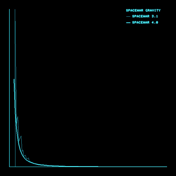
Comparative gravity plots for Spacewar! 3.1 and Spacewar! 4.x
(PDP-1 / Type 30 CRT emulation by N. Landsteiner 2014.)
Legend: x-axis: axial distance to the center (x/y), y-axis: gravity applied (see above for raw data points).
Compared with the smooth plot of version 4 the plot for Spacewar! 3.1 depicts a devil's staircase function.
We might guess by the smothness of the graph drawn by Spacewar! 4.x that this was the result of some nifty integration, like the KR4 algorithm (Kutta-Runge order 4 integration) we see employed in games nowadays, as also suggested by the name of the macro integrate. But, at closer inspection, the algorithm is quite the same as in Spacewar! 3.1. As we've observed, the jagged graph of Spacewar! 3.1's gravity function is the result of a lack of precision, caused by all the multiplications, divisions, cubes, and square root computations, which left us with just a handfull of significant bits of the initial wealth of 18-bits words. What we're seeing in Spacewar! 4.1 accordingly, is a quest for computational precision.
As stated above, we won't strive for verbal detail, but rather do with inline-comments. However, let's see how it's done:
	dzm \bx		// initially clear \bx and \by
	dzm \by
	szs 60		// check sense switch 6
	jmp bsg		// deployed, no star, no gravity
	lac i mx1	// pos x
	dac \t1
	mul \t1
	scr 1s
	dac \acx	// \acx = mx12 / 2  (high part)
	cla
	scr 2s
	dio \iox	// \iox = mx12 / 2  (low part, 2 bits zero padding)
	lac i my1	// pos y
	dac \t1
	mul \t1
	scr 1s
	dac \acy	// \acy = mxy2 / 2  (high part)
	cla
	scr 2s		// IO = mxy2 / 2    (low part, 2 bits zero padding)
	swap
	add \iox
	swap		// IO = (low (y2 / 2) + low (x2 / 2)) >> 2
	scl 2s		// shift padding/carry back into AC
	add \acx
	add \acy	// square distance (mx1 × mx1 + my1 × my1)
This is actually not that different from what we've seen in Spacewar! 3.1. We're building a square distance in the accumulator, but now we're using the built-in fixed point multiplications rather than the integer multiply by BBN. Since the mul instruction returns a 34-bit result with a high order word in AC and a low order word in IO, there's something to gain. Actually, the whole handling of the low order results in IO just contributes to a carry for the square distance currently in AC at the end of this snippet.
Follows the check for the collision with the heavy star, like in Spacewar! 3.1. In version 3.1, there was an initial shift by 11 bits to the right applied to the x- and y-coordinates, transforming them from screen-coordinates to integers (8 bits) and another 3 bits for some computational reserve. Therefor, when str was 1 in version 3.1, it's now octal 100, as 1 shifted by 6 bits to the left.
	sub str		// str: 100
	sma i sza-skp	// is it smaller than str?
	jmp pof		// yes, we collide with the star, jump to pof
	add str		// restore previous square distance
Next, we compute the cube distance by multiplying the square distance by its square root, like in Spacewar! 3.1, but this time it's framed by the macors varsft and undosft:
	varsft		// shift to AC justified left, 2 bits zero padding
	dac \t1		// \t1 = square distance justified left
	jda sqt		// get square root
	mul \t1		// \t1 = cube distance
	undosft		// undo previous justification
As the names of the two macros suggest, they are about a variable shift and the respective reverse/undo operation:
define
	varsft
	dzm \xys
	dac \t1		// store AC in \t1
	idx \xys	// \xys = 1
v2,	idx \xys	// increment \xys
	lac \t1
	scr 2s		// right shift \t1 into IO 2 bits
	dac \t1		// store it
	sza		// is it zero?
	jmp v2+R	// no, redo
	scr 2s		// do another shift
	swap		// AC justified left, 2 bits zero padding
	terminate	// \xys: number of steps
To get the most out of the 18-bit precision available in AC, macro varsft inspects the value in AC in steps of a double shift to the right. As the value in AC eventually becomes zero, the value in IO is the significant 18 bits part of the initial value in the combined AC and IO registers. After an extra shift by two bits to the right (2 bits zero padding to allow for a sign and any carry) we swap this back, with now the significant bits in AC. Variable xys stores the number of double-shifts applied. (All the storing and restoring of the contents of the accumulator in \t1 is just for the instruction idx destroying its contents by leaving the value resulting from the increment in AC.) What's now in AC, is the significant part of the initial value, justified left with a padding of two bits for some computational reserve.
Macro undosft isn't really applying the reverse operation, it adds another transformation:
define
	undosft
	dac t1		// AC in t1
	dio \t2		// IO in \t2
	lac \xys	// get number of shift steps of varsft
	add sft
	dap .+1		// set up address of according shift
	lac .		// load it and deposit it twice
	dac .+6
	dac .+6
	xor (10000	/ change scr to scl or scl to scr.
	dac \xyt	// store reverse shift in \xyt
	lac \t1		// restore AC and IO
	dio \t2
	scr .		// apply the shifts
	scr .
	terminate

sft,	lac .-1
	scr 7s
	scr 6s
	scr 5s
	scr 4s
	scr 3s
	scr 2s
	scr 1s
	scr		// "scr 0" - no shift at all
	scl 1s
We may want to go a bit more into detail here: When AC was holding just up to two significant bits, we only applied a single double-shift in varsft and variable xys would be 2. In this case, we would use the instruction at "sft -1 + 2", namely a combined shift to the right by 7 bits ("scr 7s"), just immediately below label sft, and apply this twice. In case we had to apply the full range of 9 double-shifts, we would apply the last "scl 1s" twice, and in case we applied 8 double-shifts, we won't apply any transformation at all.
As a notable side effect, we store the reverse operation of the selected shift instruction (by flipping the significant bit of the micro-code, instruction scl is 667xxx, scr is 677xxx) in variable \xyt for later use.
Back to main, we're scaling our gravitational factor according to sense switch settings:
	scr 9s		// shift 17 bits left (low gravity 15)
	scr 6s
	szs i 20	/ switch 2 for light star
	scr 2s
	sza
	jmp bsg		// overflow, apply no gravity at all
	scr 1s		// shift by another bit (complete swap with full gravity)
	dio \t1		// deposit IO in \t1
As in version 3.1, low gravity will be a quarter of normal gravity (by the divisor being 4 times as big). At the end of the operation, we've applied a full swap (by 18 bits for full gravity) and store the factor in variable \t1.
Finally, we apply our gravitational factor, so delicately derived, to the position of the ship:
	integrate mx1, \bx	// apply gravity for x, resulting delta in \bx
	integrate my1, \by	// apply gravity for y, resulting delta in \by
bsg,	...
While the first two macros were actually included just once and their being a macro was merely decoupeling the computations from the main flow, macro integrate is applied twice, once for the x-coordinate and once for the y-coordinate, storing the resulting delta in variables \bx and \by respectively. Here, we finally apply the reverse shift operation prepared in macro undosft to account for the shifts applied for left justification of the gravity factor, done to squeeze the most of precision out of the 18-bit words of the PDP-1. (We may recall that no shift will be applied, if the shift in varsft was exactly 8 bits to the right twice, and shifts will increase in number of bits to the left with a decreasing number of right shifts applied in varsft.)
define
	integrate A,B
	cli
	lac i A
	scr 9s		// AC/IO >> 10 (screen coordinates to integer >> 2)
	scr 1s
	div \t1		// divide by gravity factor
	hlt		// here on div overflow, else skipped
	cma+cli-opr	// complement AC, clear IO
	xct \xyt	// apply reverse shift ( "rcl 1s " ..  "scl 7s ")
	xct grv		// apply "gravitational constant" (sar 6s)
	dac B		// deposit result in B
	terminate
Since the positions in mx1 and my1 respectively represent an offset to the center origin, the cma instruction in "cma+cli-opr" reverts the delta in \bx and \by to the opposite direction, pulling the ship closer to the center when added to the current dx/dy movement vector. The code where this is applied, following below this at label bsg, is just the same as in version 3.1.
Generally, we may describe the procedures as converting the fixed point values (as derived from the format used by the display instruction: sign, 9 integer bits, 8 fractional bits) to floating point, proceding with the critical computations in floating point, and finally restoring the usual fixed point format.
As the comparative graph of the gravity computations in version 3.1 and 4.x shows, both functions produce nearly similar results in the mid and higher ranges. As might be expected, it's in the lower regions of the positional values that the gain in precision shows. Towards the origin, where the input values become smaller, significant bits are soon moved out of the range of precision without further preparations. But, with the data thus prepared as we've seen it here, computable information is still maintained as the function approaches the origin, as illustrated by the steady smoothness of the graph over the whole range of input data.
With a deeper analysis of Spacewar! 4.x gravity left as a home work — like arriving at an actual formula notation of the procedures involved —, we'll close here. (Note: This episode was originally published in back-to-school week.)
Next time we're going to explore the warfare in Spacewar, as in pyrotechnics and explosions.
*****
Update: A Final Note on Gravity
In case anyone would doubt a formula based on 1/r3 to be suitable for a perfect simulation of gravity, here is a professional statement on the subject, provided by Magnus Olsson, Department of Theoretical Physics of the University of Lund, Sweden at an alt.folklore.computers-thread in 1993:
>Did it ever occur to anyone that the gravity simulated in Space War (one of
>my all-time fav. computer games) is not correct
>                                    ~~~

Well, it has occured to me, but then I'm a physicist...

If classical Newtonian gravity were to wok in the same way in a 2-D
universe as in ours, the force wouldn't be proportional to 1/r^2 (r
being the distance from the "sun" to the spaceship) but as 1/r.

From this point of view, one could say that Space War doesn't
"correctly simulate gravity in a 2-D universe".

However, the matter is more complicated than this.

Firstly, Einsteinian gravity, i.e. general relativity, won't work at
all in 2 space dimensions. Either there is no gravitational force at
all, or the theory is radically different. That means that we can't
make any arguments by analogy with our familiar 3-D (or, rather,
(3+1)-D) world.

Secondly, even if one says taht we should stick to the analogy to
Newtonian gravity (i.e., to be more mathematically precise, that the
gravitational potential should be a solution to Poisson's equation in
2 dimensions) and use a force prop. to 1/r we would get problems. The
reason is that in a 1/r force field, there are no stable orbits
(except for the perfectly circular ones). This means that the space
ships would behave quite differently from the way they do in 3-space.


One might ask whether what one really wants is to simulate a truly
2-D world, or to simulate a 2-D cross section through our 3-D
universe. (I.e. we have the ordinary universe with some strange law
added that forces all space ships to keep in the plane of the ecliptic
all the time). All the space games I've seen that even attempt to have
realistic physics (most, alas, don't – space ships stop dead as soon
as you release the thrustre button, and similar atrocities) do the
latter thing.

IMHO this is a good solution, since it's the best simulation you can
get of "real" spaceflight on a 2-D screen. I find it far easier to
swallow that I'm forbidden by divine law to leave the ecliptic, but
that I can still have my familiar elliptical orbits, than to have the
strange, non-closed orbits that I would get in a true 2-D world (with
Newtonian gravity). But this is of course a matter of taste.

Magnus Olsson
Department of Theoretical Physics
University of Lund, Sweden
(Magnus Olsson, alt.folklore.computers, October 11, 1993)
*****
Vienna, September 2014
www.masswerk.at
In case you would have found any errors or inconsistencies, or would have additional information,
please contact me.
*****
◀ Previous: Part 5: Maneuvering in Space
▶ Next: Part 7: Shootout at El Cassiopeia
▲ Back to the index.