
This is a virtual DEC PDP-1 emulated in HTML5/JavaScript running some early graphics demonstrations (AKA "display hacks").
Programs available:
Explore the Test Word Switches for patterns with the Minskytron and Munching Squares!
The Minskytron must be started anew to accept fresh settings. See the button "Start".
There are various presets for the Test Word in the menu "Select a Program", listing the most common one as the main item.
Note: The Test Word Switches provide means of manual input for an 18-bit word and are located at the control console of a real PDP-1.
(Bits were counted by DEC from left to right, starting at zero for the most significant. This is also kept for the tool-tips.)
All programs are run from digital images of paper tapes to be found at bitsavers.org.
Three of these "display hacks" are combined on a single paper tape, "dpys5.rim," representing them as shown at the Computer History Museum (CHM) in Mountain View, CA. (The name "dpys5.rim" is apparently derived from "dpy", the display instruction of the PDP-1.)
The full version of Snowflake is loaded from a separate tape image named "snowflake_sa-100.bin".
Artwork and PDP-1 emulation by Norbert Landsteiner, www.masswerk.at, 2012–2022.
Based on emulation code by Barry Silverman, Brian Silverman, and Vadim Gerasimov. The original code was extended to support some additional instructions and auxilary hardware. Moreover, the shift/rotate instructions and the arithmetics were rewritten (include an emulation of the hardware multiply/divide option), and cycle counts were added for accurate timing and frame rates. Some importance was put in the recreation of the appearance of the original CRT display and the unique experience conveyed by it.
The emulator was originally conceived for running Spacewar!, the earliest known digital video game.
Play it here: www.masswerk.at/spacewar.
See also for a similar graphics demo: Graphical Fun for the PDP-1 by David Mapes.
The DEC PDP-1's Type 30 Visual CRT Display was a point plotting display* with a dual P7 phospor (light blue for fresh pixels and a yellowish green long sustain — think of radar display, this is exactly what the tubes were made for). The display featured a technical resulution of 1024 × 1024 display locations at 8 intensities, but according to DEC documentation only 512 of them on any axis were visible to the human eye. Thus, the low (or standard) resolution of the emulation, rendering at this visual resolution, is closest to real thing. (Compare the images below.) The high resolution versions render the programs at the technical resolution and are scaled down to fit the appearance of the emulated screen.
*) A point plotting display is a random access display, like a vector display, but doesn't feature any memory or line drawing capabilities. Display locations are addressed individually and have to be refreshed by the program. The long sustain of the P7 phosphor helps in keeping the image stable. The spot size of an activated display location was usually bigger than the distance between display locations, thus individual blips tended to merge. Spot sizes also varied by the intensification of the blips, bright spots were bigger than those at lower intensities.
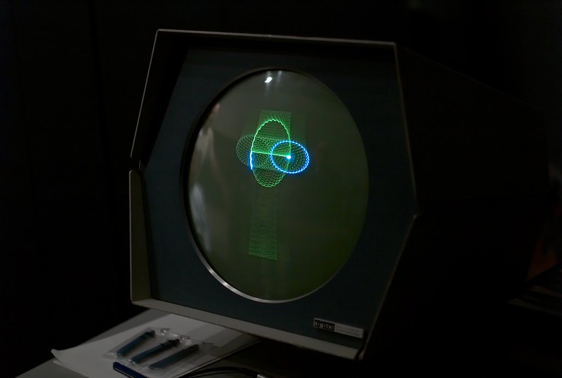
The Minskytron is a visual synthesizer based on 3 interconnected oscillators (much like a Moog synthesizer). Each oscillator advances an x- and a y-coordinate over an elliptical function, plotting a dot at the given position at each frame. The formular is based on the ancient art of drawing a circle using additions/subtractions and bitwise right-shifts (a division by powers of 2) only:
x := x − ( y >> 4 )
y := y + ( x >> 4 )
plot
repeat
(Note: This algorithm for drawing a circle was discovered by Marvin Minsky actually by a mistake that brought up a circle on the display rather than the expected curve:
“Here is an elegant way to draw almost circles on a point-plotting display:
NEW X = OLD X – epsilon * OLD Y
NEW Y = OLD Y + epsilon * NEW(!) X
This makes a very round ellipse centered at the origin with its size determined by the initial point. epsilon determines the angular velocity of the circulating point, and slightly affects the eccentricity. If epsilon is a power of 2, then we don't even need multiplication, let alone square roots, sines, and cosines! The "circle" will be perfectly stable because the points soon become periodic.
The circle algorithm was invented by mistake when I tried to save one register in a display hack! Ben Gurley had an amazing display hack using only about six or seven instructions, and it was a great wonder. But it was basically line-oriented. It occurred to me that it would be exciting to have curves, and I was trying to get a curve display hack with minimal instructions”
"Item 149 (Minsky): Circle Algorithm" in HAKMEM, Programming Hacks. (MIT AI Memo 239, Feb. 29, 1972)
The Minskytron varies this scheme by applying an individual number of right-shifts at each of these steps. (The right-shifts correspond to a divison by the given power of two, which in turn corresponds to the multiplication by epsilon, by convention a small factor less than 1, but greater than zero, as described above. Notably, shift instructions are one of the most basic and fasted instructions on a computer as compared to the more complex operations of multiplication and division, not to speak of transcendental functions, like sine or cosine, which are difficult and slow to compute.)
The respective shift instructions are derived at the start of the program from the bits of the Test Word as follows:
These shifts are then applied to the three oscillators in a round-robin fashion loop:
Rather than using the respective other coordinate of the individual oscillators, like we've seen it in the the basic algorithm for drawing a circle, here, the modifying term for a coordinate is based on the difference of this other coordinate to the respective coordinate of the next oscillator, thus connecting them in a daisy-chain. The shifts set up by the Test Word are applying an individual scaling (or distortion) to each of these factors.

The start values for the x- and y-coordinates are fixed. The Test Word provides only the means of configuring the shift instructions that are set up at the start of the program. (There is still a shift applied, if all the respective bits are set to low. All bits zero is therefor a shift by a single bit to the right, and all three bits high corresponds to an arithmetic shift to the right by 8 bits. — Thus, 0 → epsilon = 1 / 20+1 = ½ and 1 → epsilon = 1 / 21+1 = ¼, etc.)
Increasing or reducing shifts symmetrically for any pair of triple bits will change the scaling of an effect. Applying asymmetrical shifts to any pair will add distortion.
Most patterns will soon "go berserk" for the limited precision of the PDP-1's 18-bit words. — Experiment!
(An annotated version of the source code is available here.)
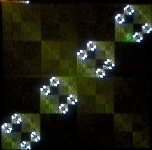
Munching Squares is a visual excercise in binary logic: Each frame starts with a reading of the Test Word. If this were either 0 or -0 (the PDP-1 represented negative numbers in 1's complement featuring the value minus zero), the octal value 2345 is used instead. This is added to the value computed in the previous frame and the result is stored. Then, the result is split in an upper and lower half by a bitwise rotation to the left by 9 bits applied to the accumulator and the IO-register as a combined 36 bit register: The higher 9 bits are transferred to the y-coordinate of the display (IO-register), but for the special format used by the display instruction — only the highest 10 of 18 bits are used — most of these bits will come into effect only at the next frame. The lower 9 bits are shifted to the most significant positions (again, there is an interleaf with a previous frame, the frame before the last frame, as the 9 highest bits previously in IO will be transferred to the lower half of the accumulator) and an exclusive OR (xor) is applied using the stored sum as an argument. The resulting value (highest 10 bits significant only), is finally used as the x-coordinate of the display instruction. After plotting a dot at the given screen position, the program starts over for the next frame.
(As may be observed, this little program is a bit more complex than it has often been described as "a trivial computation repeatedly plotting the graph
A reference to Munching Squares is found in HAKMEM, Programming Hacks (MIT AI Memo 239, Feb. 29, 1972), items 146 and 147 — just before Marvin Minsky's memo on the Minskytron —, here described in instructions for another type of computer:
“ITEM 146:
Another simple display program: "munching squares"
It is thought that this was discovered by Jackson Wright on the RLE PDP-1 circa 1962.DATAI 2
ADDB 1,2
ROTC 2,-22
XOR 1,2
JRST .-42=X, 3=Y. Try things like 1001002 in data switches. This also does interesting things with operations other than XOR, and rotations other than -22. (Try IOR; AND; TSC; FADR; FDV(!); ROT -14, -9, -20, ...)”
“ITEM 147 (Schroeppel):
Munching squares is just views of the graph Y = X XOR T for consecutive values of T = time.”
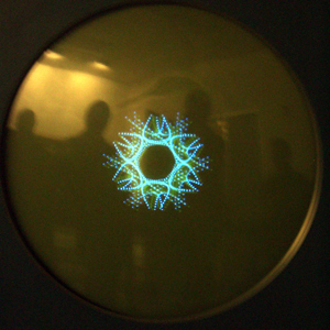
Snowflake is a graphics demo from the early to mid 1960s. Sadly, the exact date and place of origin are unknown, as is the author of this amazing little program. Snowflake displays an animated list of dots at 12 locations each, rotated over a full circle by an offset of 30° to form a starlike pattern. To do so, two lists of 56 coordinates each are initially populated by random numbers and then traversed back and forth, on each pass averaging a coordinate with its previous neighbour and displaying the result. Since the two extreme endpoints are spared from this procedure, the resulting graph is tied to these attractors, while the individual points gradually align themselves in a flowing motion. Additionally, two intermediate coordinates, one on the x-axes, one on the y-axis, are also fixed to a random location, providing two additional attractors. As the directing forces applied to the graph gradually ease thanks the avering operations, the animation slows down until a new sequence of random length starts with new random values for the two endpoints and the two intermediate attractors.
The program is here presented in two similar, but slightly different versions: Once in its the original, full form, once in the version it is shown at the Computer History Museum (CHM). The full version includes an alternative display routine, which displays the individual coordinates just as 8 dots, but drawn inside out. A further option reduces this to just a single strain, with each pair of coordinates drawn only once. (These options are available by means of sense switches 1 and 2, see the options menu ![]() or hold SHIFT and press the corresponding number key.)
or hold SHIFT and press the corresponding number key.)
Finally, there’s a third version, “Snow-Wave” (N.L., 2019), a hack of the CHM version, displaying just a single motion in order to demonstrate the algorithm. (Use sense switch 1 to toggle between this single-dot and the normal 12-dots display mode.)
See my blog for a detailed analysis and discussion of the program.
All programs are written in PDP-1 assembler code using MIT's Macro assembler.