Snowflake Archeology
Software archeology of an early computer animation (1960s) for the DEC PDP-1.
Snowflake is a small graphics program written for DEC PDP-1 somewhen in the early to mid 1960s. Its author remains to date unknow, despite all efforts, which is pretty much a pity, since s/he deserves recognition. In essence, Snowflake is a kaleidoscopic program, mapping a list of moving points multiple times onto the screen in a starlike manner. It may be even the first of these programs. However, several programmers of the day experimented with the graphics capabilities of the PDP-1 and its Type 30 CRT display, amongst them Marvin Minsky, Ben Gurley (the PDP-1’s ingenious designer), and David Mapes (see below). For sure, it’s an early specimen of the species.
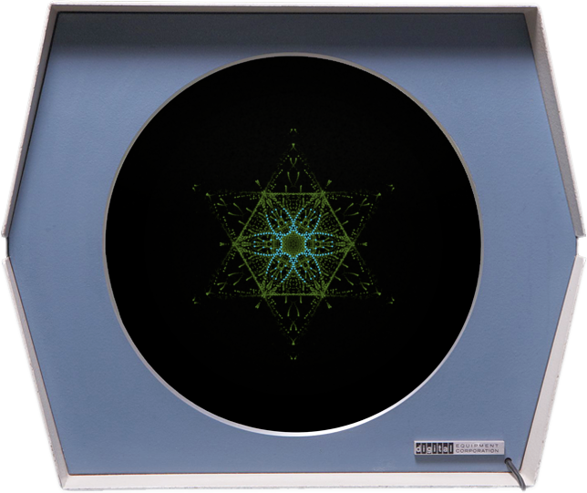
photo of Type 30 CRT display by Mark Richards, 2013.
David Mapes, who did some work on the PDP-1 at Lawrence Radiation Laboratory (at the Lawrence Livermore National Laboratory or short LLNL) himself, recalled in an oral history interview (conducted by George Michael) some of the historical impact of the program:
A program called Snowflake used this [kaleidoscopic effect] routine and was passed around to PDP-1s around the country. DEC’s president Ken Olsen got a copy when he visited the lab and took it back to [DEC] headquarters in Maynard. I’ve seen several PC screen savers using this eight-point reflection technique.
A collection of these programs was used to create a film. An offline 16mm camera was used to capture the images on the TYPE 30 CRT. An unexpected phenomena occurred when color film was used. Colors would ripple through the images displayed on the movie screen. The effect was caused by the asynchronous nature of the cycle time of the program running on the PDP-1 and the time between frames of the off-line 16mm camera. During the time the shutter was open on the camera, the points being displayed were in various stages of phosphor decay. During the next frame these points would be in another state of decay. During this decay the camera would capture the different colors during the decay, whereas our eyes integrate these colors to a single color. This film and others made using the PDP-1 at Stanford University with rented cameras were shown to various advertising executives, TV stations, the ABC and NBC networks, and the rock group, Pink Floyd. One of these films, with editing and added musical sound track, was shown to the weekly meeting of the Motion Picture Academy of Arts and Sciences in 1968, to an audience of several hundred movie professionals. The idea of computer animation had not reached the grasp of the mainstream, and I was young and scared. One of the most terrifying moments I have ever experienced was standing on the stage in front of these 200 or so movie professionals with my knees shaking, trying to answer questions from the audience and not thinking that they were understanding me.
[…]
A copy of Marvin Minsky’s Minskytron made it to the lab during the time that films were being made. I included a film segment of this in one of these films […]
And this is actually the only historic reference to the program.
Technicalities
The rippled display mentioned in the above quote refers to a peculiarity of the Type 30 CRT display, a X/Y-display, which was built around a rube originally manufactured for PPI (Planar Position Indicator) radar, for this featuring a dual P7 phosphor coating effecting in a short, bright blue activation of a newly displayed blip (also of use for a light pen) and a long, yellowish-green sustain (which helped visually stabilize things and counteracted flicker). In actuallity, the two colors would blend rother unnoticeable, but showed pretty distinct, when recorded on frame-based media, like film (or YouTube videos, by the way.)
By which we have happily arrived at the technicallities of the PDP-1. The PDP-1, announced in 1959, was somewhat a commercial version of the MIT’s experimental TX-0, the very first fully transistorized computer ever. At a comparably low price, it provided some viable computing power, suitable for real time processing, in a compact and uncomplicated package in Space Age design. The computer didn’t require a raised floor, plugged into a common wall outlet for electric power at just 120W, and could be turned instant-on by the flip of a single switch. Moreover, a display was available, which was pretty much unheard of for a commercial machine of the time.
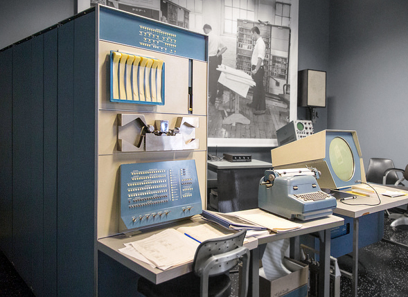
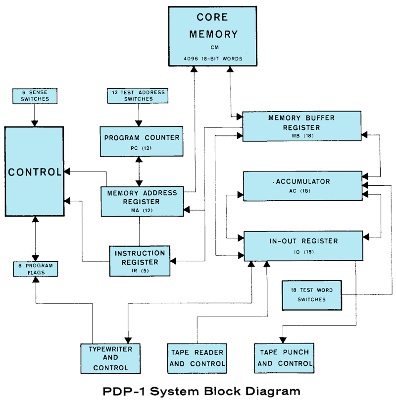
The PDP-1 was a 18-bit words machine, featured a base memory of 4K (18-bit words), which was expandable by bank switching. There were just two primary registers, the accumulator (AC) and the input/output register (IO), as well as a 6 programmable flags. For direct interaction, there were 6 dedicated console switchs, the so-called sense switches, and a full 16-bit test word register, which could be set up using a switch for each bit and could be read from inside a program. Instruction words contained both a 5-bit instruction code (at the higher end) and 12-bit addresses or operands (at the lower end.)
PDP-1 Instruction Format:


                      1 1 1 1 1 1 1 1
  0 1 2 3 4 5 6 7 8 9 0 1 2 3 4 5 6 7    bits*
┌──────┴───┬─┼─────┴─────┴─────┴─────┐
│  opcode  │i│   address / operand   │   instruction format
└──────────┴─┴───────────────────────┘

*) bits were numbered by DEC from left to right,
   starting at the most significant bit.
Regarding programming techniques, there were some interesting traits to the PDP-1: In the absence of a processor stack, in the case of a jump to a subroutine, the return address (PC+1) was put into the accumulator (AC) for the program to deal with on its own. One way to do this was patching up a jump instruction (resulting in self-modifying programs), another one using indirect addressing. For the latter, the PDP-1 featured a unversal i-bit (also referred to as delay bit), which forced a memory look-up using the contents of any memory location it was set (resulting in a possibly infinite chain of look ups, so be careful with that). On the other hand, the i-bit allowed for comfortable pointer handling, which was also greatly facilitated by a index (increment) instructions. Branching was generally done by skip instructions, which caused the program flow to skip the very next instruction in case a condition was met as true.
Runtime-wise, the PDP-1’s speed was mostly determined by its 5 microseconds memory cycle. Generally, any instructions (but multiply and divide, which were subroutines implemented in hardware and operated on their own clock) performed in 5 microseconds (200 kHz clock rate), with another 5 microseconds to be added for any memory look-up. (Since 18-bit words are much more versatile than the 8-bit byte, the resulting speed is actually faster than that of an 8-bit processor, like the 6502 at 1 MHz, used in many home computers about two decades later.)
Arithmetics were done in ones’ compliment arithmetics, representing negative numbers by just all bits flipped, which resulted in the pecularity of an additional value, minus zero, found on many early computers. (Which is, why we use two’s compliment nowadays.) For a general overview of PDP-1 instructions, see the instruction list.
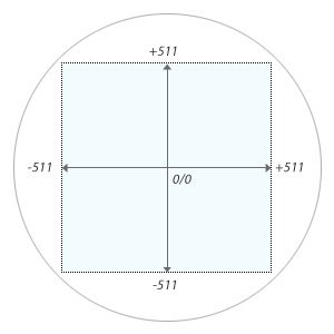
The Type 30 display, we already mentioned above, was a simple X/Y-display with a resolution of 1024 × 1024 display locations. Display coordinates were to be given in the highest 10 bits of the 18-bit instruction words, in the range of -511...+511, both for the x- and y-axis, the former in AC, the latter in IO, with the origin in the center and the negative axes pointing to the left and to the bottom. (Since this is ones’ compliment, there is also -0 and this comes just before positive 0.) As any other X/Y-display (point plotting, like the Type 30, or vector), it was an “animated” or “painted” display, meaning, displaying a dot was pretty much a fire-and-forget operation with no need to erase a point, once it was it drawn, since it faded away anyway. (If you wanted it to stay, you had to refresh it on your own.) This was pretty much for the price and speed of core memory, which made the idea of a frame buffer or video memory unpractical at the time, but also came handy for animated programs like “Snowflake”, which didn’t have to care about maintaining the screen and cleaning up behind them.
The Program
The program survived in two examples, once as binary object code (then called octal) on a paper tape called “snowflake_sa-100.bin” (“SA100” indicating a start address at location octal 100), and as in a revised version used by the CHM (Computer History Museum) for their presentations of their fully restored PDP-1. The latter is a tape named “dyps5”, comprising 3 classic “display hacks”, Munching Squares, the Minskytron, and Snowflake. The latter one is a bit simpler and also available in source code, for which we’ll mainly rely on this one for our little investigation. It’s written in PDP-1 assembler, namely for use with the “Macro” assembler, which originated at MIT. Having a look at the use of memory locations in “snowflake_sa-100.bin”, I’m personally not too sure, if this was also used for the original program.
Comparing the two programs (one in disassembly, the other one in source code), “snowflake_sa-100.bin” shows some extra jumps and a non-linear sequence of code blocks, which indicate that this program came out of an evolution of similar experimental programs, which is also assisted by the placement of some variables in an extra block, hinting at them being a later addition to the core algorithm. The main difference of the two programs, apart from some subtle differences in the patterns produced by them, is in “snowflake_sa-100.bin” also providing alternate display modes to be selected by two of the sense switches. One option is for shifting the display origin to the lower left corner (an option of the Type 30 display), thus drawing the pattern outsiide-in, rather than from the center, the other one, modifying this first option, for displaying just a single strain (or ray) of the dots, skipping the display of any mirrored dots.
The two programs are available at bitsavers.org (see dpys5.mac, “snowflake_sa-100.bin” is found in the archive InsidePDP1_80s_box3.zip) and can be explored here in in-browser emulation.
Regarding requirements, the program requires the automatic hardware multiply/divide option, which was optional for early PDP-1s (which provided just partial operations for this and had to rely on subroutines), but soon became standard (in about 1962). Since the program ran on bare metal, there weren’t any other requirements, but a display (about half of the about 50 PDP-1 installations quallified for this), which goes without saying for a visual program. So this may give a bit of a hint, but not too much of a hint, regarding the time and place of origin.

Analysis
Let’s have a look at how Snowflake does “its thing”. For the purpose, we’ll walk through the source code (as in “dyps5.mac”) from top to bottom and try to discern how things are achieved.
BTW, you can experience this version
- in in-browser emulation,
- or enjoy the real thing in video: www.youtube.com/watch?v=Y1ioLo2I_5Y,
- and in another video: www.youtube.com/watch?v=37uXPw3xF2M,
- or visit this page at DigiBarn for more authentic photos and videos.
Setup
Note: All source comments, but the very first one, are by me, N.L., and not found in the original program.)
/ start at 10 for snowflake

10/
These very first lines are both simple and cryptic as they are instructive: On the first one, we learn that anything starting with a forward slash (“/”) is a comment, and on the next line, we learn that there’s an alternative use of the slash, namely setting the program counter for the means of the assembly to the expression immediately preceeding it. In this case, we’re starting our program at 10 — and this means octal 10 (decimal 8), since all values are in octal (unless we instruct the assembler to do otherwise, which we’re not going to do in this particular program).
Generally, the assembler simply adds up anything listed in a line to form an instruction. (E.g., “1000 40” would be summed up as 1040.) Anything consisting of up to three lower-case letters or numbers followed immediately by a colon is a symbol, with appropriate values already defined in the assembler for the basic instructions. A symbol followed immediately by a colon defines a label for the current memory location.
beg,  law t1a           / load address of sym "ta1" as value into ac
      dac p1            / deposit value in ac at address p1 (used as pointer)
      law t2a           / load address of "ta2" into ac
      dac p2            / deposit at p2 (used as pointer)
At label “beg”, we meet the actual beginning of the program, starting with a little setup sequence. Instruction “law y” transfers any operand y directly into the accumulator as a literal value, in this case the address location labeled by symbol “t1a”. This is then stored by instruction “dac p1” in the memory location labeled “p1”, which will be used as a pointer later on. This is then repeated for “t2a” and “p2”. We may represent this (using C-like pointer notation) as,
p1 := &t1a
p2 := &t2a
“t1a” happens to be the beginning of an address range marked up at the very end of the program, spanning over octal 070 (decimal 56) memory locations to label “t1e” with a label “t1m” somewhere in the middle. “t2a ... t2e” mark also up a 070 words address range with label “t2m” in the middle (a dot represents the currrent address location, hence “.+23/” reserves octal 023 memory locations by advancing the program counter by the same amount):
t1a,
.+23/ t1m,
.+45/ t1e,

t2a,
.+33/ t2m,
.+35/ t2e,
The two ranges look rather similar, but differ in the position of the label placed at about the relative middle of the respective ranges. Also, “t1e” labels the same address as “t2a”, while its offset is larger by 1 than the respective offset of “t2e”. (For all practically, this incongruency of the two ranges won’t matter, since all loops are measured by the range t2a...t1e, starting from pairs of t1a / t2a.)
This might be expressed in pseudocode as,
t1a := &( word[0160] )
t1m := t1a + 023
t1e := t1m + 045        // t1a + 070

t2a := t1e
t2m := t2a + 033
t2e := t2m + 035        // t2a + 070
Hoewever, unlike in our C-like pseudocode, these are ordinary labels, which may be used like any other symbol. For congruency, we’re going to use these symbols like normal variables in pseudocode further on.
(Meaning, we’ll regard these just as variables that happen to be tied to specific addresses — which is exactly, what these are in assembler — and reserve pointer notation for an indication of indirect addressing.)
Picking up our assembler code, where we’ve left it before, we continue by:
b1,   jda cxy           / convolute x and y (p2 in ac, not used),
                        /  returns some random in ac and io
      dac i p1          / deposit ac in address in pointer p1
      dio i p2          / deposit io in address in pointer p2
      idx p1            / index p1
      idx p2            / index p2
      sas (t2e          / p2 == t2e?
      jmp b1            / no, jump to b1 (redo)
      law i 40          / load -040 into ac
      dac c1            / deposit in c1 (c1 := -040)
Here, instruction “jda cxy” jumps to a subroutine at label cxy. There are actually two mechanisms for a jump to a subroutine on the PDP-1: The common instruction “jsp”, which will put the return address into the accumulator (thus destroying any previous contents), and instruction “jda”, which additionally deposits the contents of ac for later recovery in the memory location at the given address and continues execution at the location immediately following to it as the effective jump target. Interestingly, as we will learn later, this contents of ac is never recovered, which is also true for any other jumps to a subroutine, we’ll encounter in the program.
This is much unlike any code, I’ve seen originating from M.I.T., where the PDP-1 community seems to have been deeply entrenched in hacker culture, always going for the leanest code. (“jda” comes at an extra cost of a spare memory location used to save the contents of ac and a runtime penalty of 5 microseconds.) Here, we seem to encounter a programmer who is more aligned to standard procedures, using “jda” anyway.
Note: Actually, there’s also a third mechanism for subroutines, namely “cal”, a hardwired shortcut equvalent to “cal 100”, but this didn’t enjoy much use.
We’ll care about the workings of subroutine “cxy” in a few minutes. Apparently, it convutes some values (x and y) and returns a value in ac, which is stored in the location, pointed out by the value in “p1” (mind the “i” setting the i-bit for indirect addressing). Similarly, another value is returned in io, which is stored at pointer “p2”. Currently, “p1” and “p2” are pointing to “t1a” and “t2a”, respectively, the very first locations of our two reserved 070 words address ranges.
Instruction “idx p1” (index contents of memory location) increments the address in pointer “p1 and leaves the incremented value also as a side effect in ac. Similarly, the next instruction “idx p2 advances pointer p2”. ”Instruction “sas y” skips the next instruction, if the value in memory location y is equal to that currently in ac. Since any expression in parentheses (the closing part is optional and may be omitted, like done here) marks up a constant expression, we compare the address in pointer “p2”, left in ac, to the very end of our second address range. If we reached this final address, we’ll skip the next instruction, a jump to the beginning of the block at label “b1”. Hence, we’ve just formed a loop over the two address ranges “t1a...t2e-1” and “t2a...t2e-1”, respectively, populating pairs of pointers by the values returned by subroutine “cxy”.
Note: Constants will be inserted by the assembler at the next occurrence of the preudo-instruction “constants” (nowadays called an assembler directive) and our brave little assembler will also take care of multiple occurrences of the same constant, inserting it only once and reusing the address.
Finally, “law i 40” loads a value of octal -040 into ac and deposit at label c1. (The i-bit enjoys a secondary function with a few instructions, mostly inverting the semantics, like here, where we load the ones’ complement of the operand for a negative value. Similarly, the i-bit inverts the condition of any conditional skip instruction.
We may sum this up as,
repeat {
    cxy(ac)
    *p1 := ac
    *p2 := io
    p1++
    p2++
} until (p2 == &t2e)
c1 := -40
Without giving away too much too early, we may disclose that “c1” is used as a counter for the outer loop oft the main routine, counting up to zero and determining the length of an animation sequence.
The Main Loop
Time to have a closer look at the main routine. Since we’ve now met some of the more vital instructions and concepts of the PDP-1 already, we’ll be progressing (hopefully) at some increased pace.
b2,   lac i p1          / load value in addr in p1 into ac
      dac t1            / deposit it in t1
      lac i p2          / same with p2 and t2
      dac t2
Here, we store a copy of the value pointed out by “p1” at location “t1” and do the same for “p2” and “t2”. (Obviously, some kind of working copy.) Currently, “p1” is pointing to “t1e-1” and “p2” to “t2e”.
t1 := *p1              // p1: t1e
t2 := *p2              // p2: t2e
b3,   law i 1           / decrement p1: load -1
      add p1            / add addr in p1
      dac p1            / deposit in p1
      law i 1           / decrement p2
      add p2
      dac p2
      sad (t2a          / p2 reached addr t2a?
      jmp b4            / yes, exit to b4
      jda dxy           / display it (p2 in ac, not used),
                        /  (returns ac: t1, io: t2)
      dac i p1          / deposit ac (t1) in addr in pointer p1
      dio i p2          / deposit io (t2) in addr in pointer p2
      jmp b3            / jump to b3 (redo)
The next block decrements our two pointers p1 and p2. Since the PDP-1 has an instruction for increment (“idx”) but none for decrement, we have to handle this by adding -1. The conditional skip instruction “sad y” works similar to “sas”, we’ve seen before, but will skip if the value in location y differs from that in ac. Thus, we here check for p2 having reached the start of the address range at t2a. If so, we’ll take the jump to label “b4”. Otherwise, we’ll execute a subroutine labeled “dxy”. (The initial character “d” may hint on some display routine.) Apparently, this subroutine also delivers a value in ac, which we store in pointer p1, and another one in io, which we’ll store in p2. Then, we jump back to the beginning of the block at label “b4” for another iteration.
for (;;) {
    p1--
    p2--
    if (p2 == &t2a) break;
    dxy(ac)
    *p1 := ac          // ac: new t1
    *p2 := io          // io: new t2
}
Notably, the decrement is done before any call of the subroutine “cxy”, doing the actual work. Therefore, our loop effectively calls the subroutine just for the range of t2e-1 ... t1a+1, sparing the two extremes.
The next block at label b4 is to where we took the jump, in case we met the condition in this display loop:
b4,   lac i p1          / copy value in addr in p1 (t1a) to t1
      dac t1
      lac i p2          / copy value in addr in p1 (t1a) to t1
      dac t2
Here, we save two new copies of the values pointed out by our pointers p1 and p2 in t1 and t2, respectively. Notably, the pointers are now pointing at “t1a” and “t2a”.
t1 := *p1              // p1: t1a
t2 := *p2              // p2: t2a
b5,   idx p1            / index p1
      idx p2            / index p2
      sad (t2e-1        / p2 reached addr t2e-1?
      jmp b6            / yes, exit to b6
      jda dxy           / display it
      dac i p1          / deposit ac (t1) in addr in pointer p1
      dio i p2          / deposit io (t2) in addr in pointer p2
      jmp b5            / jump to b5 (redo)
This is similar to the block, we’ve seen before at “b3”, but this time we’re incrementing up towards the last valid pointer address at “t2e - 1” for another display loop starting with values for t1 and t2 as last used inside the first display loop (actually the same values as stored in t1a+1 and t2a+1 as we enter this second loop).
for (;;) {
    p1++
    p2++
    if (p2 == &t2e - 1) break;
    dxy(ac)
    *p1 := ac          // ac: new t1
    *p2 := io          // io: new t2
}
To sum this up, after the setup, we enter a first loop, decrementing from t1e / t2e towards t1a / t2a and calling subroutine dxy for the ranges t1a+1...t1e-1 and t2a+1...t2e-1. In the process the values inside this ranges are updated, as well. The same is then done in the other direction, but now just affecting the ranges t1a+1...t1e-2 and t2a+1...t2e-2, sparing t1e-1 and t2e-1.
Locations t1a and t2a, as well as t1e and t2e, are left untouched by the two loops. (However, t1e is the same address as t2a.)
As we’ve reached the end of the second display loop, we continue at label “b6”:
b6,   isp c1            / index c1 and skip next if positive
      jmp b8            / c1 < 0? jump to b8
      jda cxy           / convolute x, y
      dac t1a           / deposit ac in t1a
      dio t2a           / deposit ac in t2a
      jda cxy           / convolute it again
      dac t1e-1         / deposit ac in t1e-1
      dio t2e-1         / deposit ac in t2e-1
Instruction “isp y” (index and skip if positive) increments the value in location y, just like “isp” does, but also skips the next instruction, if the resulting value is positive. Combined with a jump instruction it provides a perfect iterator for a count-up towards zero. Here, we increment “c1”, initially set to -040. In case, it’s zero or any other positive value after the increment, we skip the jump to label “b8” and set up a new animation sequence. To do so, we set up new value pairs in t1a / t2a and t1e-1 / t2e-1 by means of our enigmatic convolution routine at “cxy”. (Otherwise, while continuing a sequence, the two display loops will reuse the same starting values for t1 and t2.)
if (++c1 >= 0) goto b8
cxy(ac)
t1a := ac
t2a := io
cxy(ac)
(&t1e - 1) := ac
(&t2e - 1) := io
Obviously, this is meant to supply some (allegedly) random numbers to the two pairs (t1a/t1e-1) and (t2a/t2e-1) at both ends of our actual working ranges. But, didn’t the first display loop also affect t1e-1 and t2e-1? As we’ll see in a second, no further changes are applied to the two pointers p1 and p2 and we’ll renter the main loop with values just as they are now. but these are currently pointing to t1e-1 and t2e-1, respectively, meaning, any further iterations of the display loops (but the very first one, just after the start of the program) will consistently only affect the ranges t1a+1...t1e-2 and t2a+1...t2e-2. So, indeed, these two pairs are outside the affected ranges, bracketing them on either ends.
There are just a few instructions left in this particular strain:
b7,   jda cxy           / convolute it again
      dac t1m           / deposit ac in t1m
      dio t2m           / deposit io in t2m
      jmp b9            / jump to b9
Here we’re still continuing the setup of a new sequence. Again, we get us another pair of convoluted values and store it in locations t1m and t2m, which are located roughly in the middle of the respected ranges. As far as we’ve seen by now, there is nothing special obout them, since the two displays loops are iterating over them like any other items in the two lists.
cxy(ac)
t1m := ac
t2m := io
goto b9
At label “b8”, we’re picking up the strain, which diverted for a normal continuation of a sequence (c1 < 0):
b8,   lac x             / load x into ac
      dac t1m           / deposit ac in t1m
      lac y             / load y into ac
      dac t2m           / deposit it in t2m
      jmp b2            / jump to b2 (redo main loop)
Here, we also set t1m and t2m, but this time to the values currently hold in x and y, respectively. We haven’t seen those symbols yet and they are used by the routine at “cxy” exclusively. (We really ought to have a look at this one soon.) With t1m and t2m thus set up, we jump to label “b2”, the entrance of the main loop.
t1m := x
t2m := y
goto b2
In case we were setting up a new sequence, we’re still in the race, at label “b9”, precisely:
b9,   and (74           / ac (t1m) AND 0b111100
      cma               / complement ac (negative)
      dac c1            / deposit it in c1
      jmp b2            / jump to b2 (redo outer loop)
Here, we set up a new value in c1, the counter used to determine the duration of the main loop. For this, we first AND the value in ac (which was last the same as in t1m or x) with octal 074 (provided as a constant expression). 074 happens to be in binary representation 111100, meaning, provided any of those bits are set, it will be a multiple of 4 at a maximum of decimal 60 iterations. Since we’re going to count up on this value, we complement the value in ac by instruction “cma” to get the respective negative value (ones’ complement, all bits flipped) before storing it in c1. Finally, we jump to “b2” to redo the main loop.
c1 := ac AND 074
goto b2
And this was the main loop. Following a tiny setup sequence for an initial population of the two lists at “t1a” and t2a, it loops back and forth over the two lists, calling subroutine “dxy” for each iteration. This subroutine also provides some kind of iteration for the list items, which are updated in each iteration. Finally, the two items t1m and t2m at about the middle of the two lists are reset to new values. The outer loop counter c1 is incremented, and, if it happens to be zero, new values for the extreme ends of the two lists are optained and c1 is asigned a new, apparently random value.
We may observe a small inconsistency in this, as the very first execution of the first display loop extends over an extra item, which isn’t visited thereafter. Anyway — now we really ought to have a look at the enigma, which is routine “cxy”.
Convolutions — cxy
cxx,  0                 / return address

cxy,  0                 / ac dumped here (not used)
      dap cxx           / point of entry: deposit return address
      lac x             / load x
      mul (362643       / muliply by 0362643
      rir 1s            / rotate io (minor result) right 1 bit pos
                        /  (reposition sign bit in io17 to io0)
      dio x             / deposit it in x
      lac y             / load y
      mul (362643       / same as above, store minor result in y
      rir 1s
      dio y
      add x             / add x to major (most significant) part
      dac x             / deposit it in x
      rcl 4s            / rotate combined ac and io left 4 bits
      jmp i cxx         / return
As we enter this subroutine by “yda cyx”, the contents of ac becomes dumped at address cxy and execution starts at the next address. Here, we dump the return address, which is now in ac, into the location labeled “cxx”. (Labeling a return address by the same prefix as a subroutine but ending in the letter “x” is a convention, which may be observed in many PDP-1 programs. However, this is also dissimilar to most code that originated at M.I.T., where usually the address part of a final jump instruction was fixed up by instruction “dap”, as in deposit address part, which saves 5 microseconds for an indirect look up, as used here as the very last jump.)
Anyway, the “body” of our routine starts with loading the value at label “x” into ac. “x” is initially set to 0520063, negative number. Next, this number is multiplied by the constant 0362643 by the instruction “mul (362643”.
Here, we have to know how “mul y” actually works: As the name indicates, it multiplies the value in ac by the value in location y (here implicitely provided by the assembler constant). Both 18-bit words are regarded as signed 18-bit values, consisting of a sign bit and a 17-bit fractional part, representing a fractional number with the “decimal point” immediately after the sign bit. The multiplication results in a 34-bit value, which is provided as major part in ac and the minor, less significant part in io. This 34-bit value is padded on both ends by a sign bit, in bit 0, the usual sign position for ac and bit 17, the least significant bit in io (By this, the result is returned in a well formed 36-bit format, which also preserves the sign separately for the minor part in io.)
Our subroutine now stores the minor or least significant part (as returned in io) back in location “x”. However, in order to do so, this value has to be transformed into an ordinary number format, which is achieved by “rir 1s”, a simple bitwise rotation to the right by a single bit position. (The PDP-1 has a barrel shifter, supporting shifts by multiple bit positions at once. The amount is here provided by the assembler symbol “1s”, indicating a single bit position. Moreover, bits lost at one end reenter immediately at the other end, as there is no dedicated carry or link flag to act as intermediary storage.) Thus prepared, we store the value by “dio x”.
The same procedure is then repeated for the value in y, which is initially set to 0350735. This time, we also make use of the major, most significant part of the new “y” and add it to “x” and store the updated value.
Finally instruction “rcl 4s” performs a rotation to the left by 4 bit positions on the combined ac and io register, acting as a 36-bit register (just as it did for the result of the multiplication). This is bit peculiar: A simple shift to the left by 4 bits would be equal to a multiplication by decimal 16. However, at the same time,the rotation also shifts the upper 4 bits from the respective other register into the lower 4 bits, thus combining parts of unrelated values.
To all respect, we may interpret this as some kind of scrambling operation. At the same time, we may regard this still as a multiplication by 24 modulo 218, populating the resulting empty space by some random bits, whith the side effect of a random change in signs (depending on the state of what was previously bit 4, counting from the MSB). There’s still some kind of numerical relation.
In pseudocode this may be described as:
sub cxy(dummy_argument) {
    mul(x, 0362643)
    x := (io >> 1) OR ((io AND 1) << 17)
    mul(y, 0362643)
    y := (io >> 1) OR ((io AND 1) << 17)
    x := x + ac                          // 18 bit!  x = x AND 0777777
    // rcl 4s:
    uint36 t = ((ac AND 0b000011111111111111) << (4 + 18))
               OR (io << 4)
               OR (ac >> 14)
    ac := t >> 18
    io := t AND 0777777
    return
}

sub mul(a, b) {
    // |a| < 1, |b| < 1
    bit    s1 = sign(a)
    bit    s2 = sign(b)
    uint34  r = |a| × |b|
    ac = r >> 17
    io = ((r AND 037777) << 1)
    if (s1 != s2) {
        ac := -ac
        io := -io
    }
    return
}
So, what is this multiplication all about? We may obsserve that the addition “x := x + y” overflows from positive to negative and vice versa, if the result exceeds a signed 18-bit value. We may note this for later.
Ignoring the construct “rcl 4s” at the very end, the whole subroutine reminds of an algorithm discoverd by Marvin Minsky (and used in his Minskytron program), which he described as follows:
Here is an elegant way to draw almost circles on a point-plotting display:NEW X = OLD X – epsilon * OLD Y NEW Y = OLD Y + epsilon * NEW(!) XThis makes a very round ellipse centered at the origin with its size determined by the initial point. epsilon determines the angular velocity of the circulating point, and slightly affects the eccentricity. If epsilon is a power of 2, then we don’t even need multiplication, let alone square roots, sines, and cosines! The "circle" will be perfectly stable because the points soon become periodic.
The circle algorithm was invented by mistake when I tried to save one register in a display hack! Ben Gurley had an amazing display hack using only about six or seven instructions, and it was a great wonder. But it was basically line-oriented. It occurred to me that it would be exciting to have curves, and I was trying to get a curve display hack with minimal instructions.
“Item 149 (Minsky): Circle Algorithm” in HAKMEM, Programming Hacks. MIT AI Memo 239, Feb. 29, 1972)
The same algorithm was independently discovered by David Mapes, who described it as follows:
One day when Roger Fulton was leaving for home, he said that what would really impress him would be if he could come back tomorrow and find a circle displayed on the TYPE 30 CRT. Later that night, I lay in bed thinking about this when it occurred to me that subtracting a fraction of the current y value from x and adding a fraction of y to x would create the next point on a circle. I strained to visualize this for different values of x and y. It would hold for the 8 values at each 45 degrees but it was hard to visualize other values. I jumped from bed and headed for the lab and the PDP-1. I arrived around 2:00 am and wrote a small program that would do arithmetic shifts to divide x and y by 16 and compute x = x + y/16 followed by y=y-x/16 then display the resulting point and repeat the process. And there it was: a circle on the display. I was so excited that I started playing with it, adding to the program, generating ellipses, and didn’t leave the consol of the PDP-1 until 2:00 am the following morning. Needless to say, when Roger arrived, he was impressed. By the time I got back to the lab the following day, Chuck Leith met with me and gave a complete description of the algorithm with details about the maximum deviation from a perfect circle and how to determine the number of points needed to complete a circle. I was impressed that he could come up with so much information about this and in such a short time. Later, it occurred to me that Chuck Leith and I should have published this work. Shortly after that, George Michael made me aware that I had rediscovered what was discovered long ago.
The following is this program using multiplies instead of arithmetic right shifts. It is written for a PDP-1. It uses two variables, c1 and c2, for the multipliers, where c1 = -c2, so that no subtract is done. This is done to provide the ability to generate different conic sections without changing the program.
Variables with initial valuesProgram
- x= 0
- y=+32 = Octal 040000
- c1=1/8 = Octal 040000
- c2=-1/8 = Octal 737777
- For a circle c1 = -c2
- For an ellipse c1 is not equal to c2 and the signs must be different
- For a hyperbola quadrant the signs c1 and c2 are the same but the magnitudes can vary.
Loop:       Lac  y
            Mul  c1
            Add  x
            Dac  x
            Mul  c2
            Add  y
            Dac  y
            Lio  y
            Lac  x
            Display point (x,y) on CRT: no need to wait
I used variations of this program in conjunction with other graphic algorithms to create many animated graphic displays. There was a routine that would take a point x and y and create seven more points:Displaying these eight variations for a list of points creates a kaleidoscopic effect on the display. A program called Snowflake used this routine and was passed around to PDP-1s around the country. (…)
- P(-x,y)
- P(y,-x) swap x and y
- P(-y,-x)
- P(-x,-y) swap x and y
- Px,-y)
- P(-y,x) swap x and y again
- P(y,x)
David Mapes in “A Statement from David Mapes”,
at www.computer-history.info – Stories of the Development of Large Scale Scientific Computing at Lawrence Livermore National Laboratory; An oral and pictorial history compiled by George A. Michael (and others)
Now, especially David Mapes’ representation of the algorithm bears some semblance to our “cxy” routine. However, there are also differences: While Mapes treats the multiplication as an integer operation (as does Minsky by using shifts in his Minskytron), the multiplication is used here in its documented manner of an multiplication of fractional factors and only the minor part of the result is used (as opposed to the major part in ac by Mapes). However, “x” and “y” are not used directly as display coordinates in our case, they are just some factors.
Maybe more crucially, the first term isn’t added to (or rather, subtracted from) the other factor (which should be “y” in our case), rather, “y” is just receiving the (partial) result of the multiplication. Still, we may still discern the pattern, even if it’s in derivative or distorted form, a rotor of sorts. This is still true, even, if there is no subtraction, since the addition is likely to overflow eventually. Regarding functional properties, we may speculate that this may result in some kind of closeup on a section of a distorted circle, plotting a wavelike motion.
We may speculate that word had spread of Mapes’ discovery, but was not rightly understood as by using just the minor part of a fractional multiplication result, which was followed by some further tweaks to the routine. (In this case, we may assume that David Mapes’ similar experiments may have been first.) On the other hand, similarities may be just coincidental and this was yet another independent discovery and/or the effect was just what had been intended from the beginning. A probable counterargument may be found in the last scrambling operation “rcl 4s”, which delivers the values actually used by other parts of the program and reminds more of a correction or the result of experimentation. Probably, we’ll never know.
Since the numerical analysis required for further inspection is far beyond my expertise, I’ll treat it as what it obviously is, a convolution of sorts involving values x and y, delivering some scrambled factors in ac and io to be used to populate the two lists.
Heavy Display Lifting — dxy
By this we’re left with routine “dxy” to explore, which pbviously does more than just displaying a dot. It spans over about one and a half pages and starts like this:
dxx,  0                 / return address

dxy,  0                 / ac dumped here (not used)
      dap dxx           / point of entry: deposit return address
      szo               / overflow flag zero? implicitely clears ov-flag
      cla               / no. dummy instruction: clear ac
      lac i p2          / load value in addr p2 into ac
      add t2            / add t2
      szo               / overflow?
      jmp dx1           / yes, jump to dx1
      sar 1s            / shift ac right 1 bit
      jmp dx2           / jump to dx2
Like we’ve seen it above at “cxy”, we start by storing the return address. Next we check the overflow flag by instruction “szo” (skip on zero overflow). If this flag is zero, we skip the next instruction, “cla” (clear accumulator), which will reset ac to zero. The overflow-flag (ov) is maintained internally by the PDP-1 and the instruction “szo” only means to access it. This will not only check the state of the flag, but also reset it to zero. What is exactly, what it is here used for. “cla” is merely a dummy instruction, since the very next, unconditional instruction, “lac i p2” is setting ac, as well. This one loads the value from pointer p1 into ac and t2 is then added to this.
Here, we encounter another “szo” instruction, which is now used in ernest: If an overflow occured in the previous addition (it must have occured there, since we implicitly cleared the flag just before), we won’t skip the next instruction and will take the jump to label “dx1”. If the overflow-flag was zero, we’re still in business and execute the arithmetic shift to the right by 1 bit position as in “sir s1”, effectively a divide by 2. Then, we jump to the next block at label “dx2”.
However, if an overflow occurred, we continue at “dx1” as follows:
dx1,  xor (377777       / flip all bits but sign
      sar 1s            / shift right 1 bit
      xor (577777       / flip all bits, but original sign bit (bit 1)
This also executes a shift to the right by a single bit position, but also corrects the sign bit lost in the overflowing condition. We may reconstruct this from the bit now in sign position, resulting from the addition of the sign-bit with the overflowing carry. If it is now set, it must have been unset (positive) before, else, it must have been a negative value. Either way, we want the sign bit after the shift to be the exact complement of what it is now. One way to achieve this, is to complement all bits but the sign bit (bit 0) before the shift as in “xor (377777”. Since the bit newly shifted in by the arithmetic shift is a copy of the previous sign bit, we now have to flipp all bits again, including the sign bit, but excluding the previous sign bit (now bit 1), as in “ xor (577777”.
(We may note that the same could have been achieved just by the shift followed by a simple flip of the sign bit, as in “xor (4000000”, as well.)
sub dxy(dummy_argument) {
    ov := 0
    ac := *p2 + t2
    if (ov) {
    	ov := 0
        // shift and restore sign
        ac := ac XOR 0377777
        ac := ac >> 1
        ac := ac XOR 0577777
    }
    else {
        ac := ac >> 1
    }
At label “dx2” both strains reuinite again with the shifted sum in ac:
dx2,  dac t2            / deposit ac in t2
      lac i p1          / load value at addr in p1
      add t1            / add t1
      szo               / overflow?
      jmp dx3           / yes, jump to dx3
      sar 1s            / shift right 1 bit
      jmp dx4           / jump to dx4

dx3,  xor (377777       / handle overflow
      sar 1s
      xor (577777

dx4,  dac t1            / deposit in t1
      lio t2            / load t2 into io
Here, we finally store the result in t2. The next instructions are just the same as we’ve seen them before, but now for adding the value of pointer p1 to t1 and shifting the sum (with a possible correction of the sign bit). The new value is then stored in t1 and the previous one loaded from t1 into io.
    t2 := ac
    ac := *p1 + t1
    if (ov) {
    	ov := 0
        // shift and restore sign
        ac := ac XOR 0377777
        ac := ac >> 1
        ac := ac XOR 0577777
    }
    else {
        ac := ac >> 1
    }
    t1 := ac
    io := t2
So far, we’we updated the pairs of values in t1 and t2 by the sum with the pointers in p1 and p2 devided by 2. These are exactly the two values t1 and t2, which will be returned without further changes in ac and io. Notably, as we’ve already seen, these will be stored in the same pair of pointers p1 and p2 in the display loops.
Therfore, after this iteration, t1 equals *p1 and t2 equals *p2. However, as we enter the routine, t1 and t2 will contain the values of the previous pair: We’re effectively averaging a pair of list items (or coordinates) with the previous one and store the results for use by the next iteration. As we are walking through this in either direction, it’s effectively a smoothing operation.
Notably, when we start a new “sequence”, the values at the “ends” (t1a, t2a, etc) and the values at the “middles” (t1m and t2m) will be unrelated to this, dragging the other items towards their relative offset. What may be expected from this is a curve or wave, defined by the by 4 points at the two ends and two intermediary points (as t1m and t2m are not symmetrical), which eventually aligns itself towards a straight line.
We may also note, how the pair of values are now held in ac and io, just as they are used canonically to represent display coordinates (x and y respectively) for the display instruction “dpy”. (We may recall that the display instruction uses ac for x and io for y, where only the highest 10 bits are used as signed display coordinates with the origin in the center.)
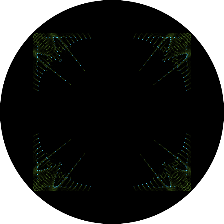
We may put this also to a test, displaying the coordinates as-is and jump to the end of the routine. And, in deed, we see a figure, defined by 4 points along a curve, which are dragging the other points, as stored in our two lists, in some kind of animated wave, a smooth operation, which also excerts some force on these 4 points:

Test run displaying just at the bare coordinates.
Mind the wave-like form defined by 4 points, one at each end and two around the middle.
As may be expected, more force is excerted on those dots which are diverging more from the average line, resulting in a greater speed of animation (visible by the longer trails).
You may experience this little hack — I called it ”Snow-wave” — yourself, as it is also available in emulation.
(Use sense switch 1, available either by the options-menu at the top right of the emulation or by holding the SHIFT+1 to toggle between the single-dot display and the normal animation.)
The result is already pleasing and even majestic, as the sequences change like tides, the extreme ends shooting off rapidly, dragged by the two invisible endpoints (t1a/t2a and t1e-1/t2e), as are the two middle points, but eventually damped by the other points, which follow smoothly, but at a slower pace behind, striving for an equalizing relief of stresses. — Actually, it’s kind of a spring embedder with quit some damping applied!
Moreover, we may assess already that the animation is effected by this smoothing operation in “dxy” and that the “convolution” in “cxy” serves just the purpose of a random number generator.
So far we may describe the overall workings (with some idealization) as follows: Two lists of coordinates are set up at startup and populated by random values. A sequence counter (c1) is set up for an initial duration of 040 “frames”. For each “frame”, two display loops iterate back and forth over the coordinates lists (excluding the two extreme ends) and update the stored values by averages with the previous pair. (Also, dots are displayed for each pair in the process.) At the end of a sequence, new random values are stored at both ends of the list and at a single x-coordinate (t1m) and a single y-coordinate (t2m) near the middle of the list (but with some asymmetric offset to the exact middle). Finally, a new duration of max 074 “frames” is determined by random and the outer loop restarts.
However, coordinates t1m and t2m will also be set in any normal iteration of the main loop (which is not starting a new sequence) to values x and y maintained by the convolution routine cxy. As this routine isn’t called during the period of an animation sequence, these coordinates will be effectively tied down in a fixed position like a split center. (We may note that this will be overwriting the random coordinates inserted there at the start of a new series or sequence, which may result in some distracting spray dots, maybe the only major flaw of the program.)
Regarding dynamics, these are achieved by assigning new random coordinates for the two ends of each list and additionally assigning just a single new coordinate for two intermediate points (one receives a new x-coordinate, the other one a new y-coordinate). The smooth, flowing motion is then achieved by releasing the resulting tension by means of averaging coordinates, thus gradually minimizing the offsets. Since the two endpoints are excluded from any modifications, the visible ends of the resulting plot will shoot off in the directions of these attractors and are soon effectively tied to their position, excerting force on their neighbors, dragging the plot behind. Thanks to the averanging applied the graph will tension between these endpoints, by this also easing the distortion effected by the two intermediate “semi-attractors”. As the offsets gradually minimize, the forces directing the graph will cool down, causing the animation to eventually slow down alike as the graph approximates an equilibrium of “forces” (which are just differences in offsets of adjacent pairs of coordinates.)
However, we haven’t display any in the unaltered program yet. And we have still to learn, how the mirroring is actually achieved. This is, were we meet label “cy1”, following immediately where have left the code previously:
dy1,  dac z1            / deposit ac (t1) in z1
      dio z2            / deposit io (t2) in z2
      sar 1s            / shift ac right 1 bit (div 2)
      dac t3            / t3 := t1/2
      lac z2            / load z2 (t1) into ac
      sar 1s            / shift ac right 1 bit (div 2)
      dac t4            / t4 := t2/2
      lac z1            / load z1 (t1) into ac
      mul (335546       / multiply by 0335546
      dac q1            / deposit in q1 (t1 × 0335546)
      lac z2            / load z2 (t2) into ac
      mul (335546       / multiply by 0335546
      dac q2            / deposit in q2 (t2 × 0335546)
      lac q1            / load q1
      sub t4            / subtract t4
      dac r1            / r1 := t1 × 0335546 - t2/2
      cma               / complement
      dac r2            / r2 := -r1
      lac q1            / load q1
      add t4            / add t4
      dac r3            / r3 := t1 × 0335546 + t2/2
      cma               / complement
      dac r4            / r4 := -r3
      lac q2            / load q2
      sub t3            / ac := t2 × 0335546 - t1/2
      lio r3            / load r3 into io
This may be a bit intimidating, but it is actually quite straight forward. First, we store working copies of t1 and t2 in z1 and z2, respectively, by this isoliting this part of the code and inhibiting any side effects. Then, we derive some factors from our coordinate pair:
    z1 := t1
    z2 := t2
    t3 := z1/2             // t1/2 = t1 × sin(30)
    t4 := z2/2             // t2/2 = t2 × sin(30)
    q1 := z1 × 0335546     // t1 × 0335546 = t1 × cos(30)
    q2 := z2 × 0335546     // t2 × 0335546 = t2 × cos(30)
    r1 := q1 − t4          // t1 × cos(30) − t2 × sin(30)
    r2 := -r1
    r3 := q1 + t4          // t1 × cos(30) + t2 × sin(30)
    r4 := -r3

    ac := q2 − t3          // t2 × cos(30) − t1 × sin(30)
    io := r3               // t1 × cos(30) + t2 × sin(30)
The multiplication by the constant 0335546 applies a scaling factor, as does the shift to the right, basically a division by 2. Moreover, octal 0335546 is binary 0b011011101101100110, which, if interpreted as a fractual numer (as done by the multiplication), looks very much the same as the cosine of 30° (which happens to be also the sine of 60°). Similarly, we may interpret the divide by 2 as a multiplication by the sine of 30° (or the cosine of 60°). — This is actually good old trigonometry!
       ┌                 ┐
       | cos(θ)  −sin(θ) |
R(θ) = |                 |
       | sin(θ)   cos(θ) |
       └                 ┘

x’ = x × cos(30°) − y × sin(30°)

y’ = x × sin(30°) + y × cos(30°)


*) Mind that ac is actually displayed as the x-coordinate
   and io as the y-coordinate.
At the end of this block, we finally load actual display coordinates into ac and io. This is still similar to the coordinates as stored in (t1 / t2), but applies a mild distortion. (If we decided to abbort the subroutine just after the first display command, the animations weren’t that much different from what we’ve witnessed already in our little test-setup.)
Time to actually display some:
dy2,  dpy 300           / display at x: ac, y: io (at intensity 3, brightest)
      cma               / invert x
      dpy 300           / display it again
      cma               / invert x again (as before)
      lio r4            / load r4 into io (y-coor)
      dpy 300           / display it
      cma               / invert x
      dpy 300           / display it
      lac t3            / load t3 into ac
      add q2            / ac = t2 × 0335546 + t1/2
      lio r1            / load r1 into io (y-coor)
      dpy 300           / display it
      cma               / invert x
      dpy 300           / display it
      lio r2            / load r2 into io (y-coor)
      dpy 300           / display it
      cma               / invert x
      dpy 300           / display it
      lac z2            / load z2 into ac (t2)
      cma               / complement
      rcl 9s            / swap io, ac
      rcl 9s            / -z2 now in io
      lac z1            / load z1 into ac (t1)
      dpy 300           / display it
      cma               / invert x
      dpy 300           / display it
      lio z2            / load z2 (t2) into io (y-coor)
      dpy 300           / display it
      cma               / invert x
      dpy 300           / display it
      lac t1            / load t1 into ac
      lio t2            / load t2 into io
      jmp i dxx         / return
Since the origin is at a center, the compliment of the x-coordinate will mirror the display location by the y-axis. With a bit of creative complementing and swapping applied, we arrive at 12 distinct “dpy” operations for any pair of coordinates, effecting an equal amount of activated blips on the screen, at the highest of the 8 available brightnesses. A rotation by 30° in 12 steps by means of what is the equivalent of a rotation matrix.
Notably, each dot is averaged and displayed twice a “frame” (i.e. iteration of the main loop) and there are 24 “living dots” displayed for each pair of coordinates.
Note: Displaying a dot on a X/Y display like the Type 30 CRT display is actually a time consuming matter, since the display has to provide for arbitrary movements from one plot location to the next. In order to maintain precision and to counteract overshoot and oscillations, which may result in a fuzzy display image, the Type 30 display engages special circuitry for cooling and activates its cathod ray only when the coils have cooled down, which takes 45 mircoseconds, or, combined with the display instruction, 50 microseconds in total. Taking this into account, the “dpy” instruction has both synchronous and asynchronous modes, either firing blindly, or requesting a “completion pulse” from the display for which the program may wait later, as well as a fully synchronous mode where the machine will stop and wait for the display to send its completion pulse. The “dpy” instruction as used here is the latter, fully asynchronous one, which is also the slowest mode of employment.
Finally, we load the undistorted coordinates into ac and io and are ready for the jump to return as in “jmp i dxx”.
    // x (ac) = q2-t3, y (io) = q3
    display(  q2 - t3,  q3 )
    display( -q2 + t3,  q3 )
    display(  q2 - t3,  r4 )
    display( -q2 + t3,  r4 )
    display(  t3 + q2,  r1 )
    display( -t3 - q2,  r1 )
    display( -t3 - q2,  r2 )
    display(  t3 + q2,  r2 )
    display(       z1, -z2 )
    display(      -z1, -z2 )
    display(      -z1,  z2 )
    display(       z1,  z2 )
    ac := t1
    io := t2
    return
}
Follow the definition of the memory loactions and their labels, as well as the pseudo-instruction “constants”, where the assembler will insert the constant taht are used in the program. The very last bit reserves the memory range for our two lists with according labels, just as we’ve seen it already at the beginning of our walk-through.
x,    520063
y,    350735

p1,   0
p2,   0
c1,   0
t1,   0
t2,   0
t3,   0
t4,   0
z1,   0
z2,   0
q1,   0
q2,   0
r1,   0
r2,   0
r3,   0
r4,   0

constants

t1a,
.+23/ t1m,
.+45/ t1e,

t2a,
.+33/ t2m,
.+35/ t2e,


start beg
The very last pseudo-instruction, “start” followed by an optional start address, ends the program and causes the assembler to insert an appropriate jump to the start of the program (here at label “beg”) at the end of the binary loader sequence it will produce.
And this was actually “Snowflake” — I hope, it was fun!
Snowflake SA-100
As this has become rather long already, we won’t go too much into detail here regarding the original program. The most intersting side to it is probably its “texture”, which shows all the signs of experimentation: Code blocks are intermingled, there’s much more jumping to and fro, bridging over unused memory location or dead code. Some locations used as variables are even located just between two blocks of code, adjacent to other, unused memory locations, which may have once served a similar purpose. Also, what are inline constants in the code as we’ve seen it in the CHM-version, are just memory locations among others used for variables, hinting at the use of an assembler which didn’t support this feature. Moreover, some of these are addressed indirectly, like the start addresses for the lists, so that these may be relocated easily.
However, there are even more telling organizational traits to the program, namely in the placement of the memory locations used for variables and the lists of coordinates: Most of them are included just before a display routine “dy1”, which is much like we’ve seen it here. Enclosed in this, we find another block of variables, namely those used for the matrix transformations, along a short block of dead code, followed by the actual 12-dot display routine “dy2”. Far beyond this (about half into the block of 4K memory), we eventually find another block of variables, mostly connected to the second list of coordinates (like t2e, t2a, p2) followed by the list itself. Maybe this is stressing thin evidence a bit too much, but we may be tempted to conclude that there was just a single list of coordinates once, with the second one included later in the course of experimentation.
Similarly, there’s another, totally different display routine, which may be actually selected by one of the sense switches, effecting in an 8-dots display. As this is located before the first block of variables, it may even have been the original one. Anyway, it may be worth risking a closer look.
Another Display Routine
So, here its is, in disassembly. The code picks up just as we’ve seen it, with the avering of the *p1 with the previous, adjacent coordinate in t1. However, at label “t4”, just as we stored t1, with the value still in ac, and expect to load t2 into io, we detour to label “dy1”, just to find the missing “lio” instruction there. — This looks much like a later insertion or patch.
Just after we executed our missing “lio t2”, we encounter an instruction “szs 20”. This is is an instruction to check the sense switches, with the number of the switch specified in the second lowest octal position. “szs” will skip the next instruction, if the regarding switch is zero (in low position). If it is high, we jump back to just after where we left, to label “dx5”, else, we continue with setting up the factors for the 12-dots transformations.
Addr.     Instr.     Disassembly

00236     240401     dx2,  dac t2
00237     210414           lac i p1
00240     400400           add t1
00241     641000           szo
00242     600245           jmp dx4
00243     675001           sar 1s
00244     600250           jmp dx4

00245     060410     dx3,  xor k4     / 377777
00246     675001           sar 1s
00247     060411           xor k5     / 577777

00250     240400     dx4,  dac t1
00251     600505           jmp dy1    / detour to dy1

/ start of alternative display routine

00252     727007     dx5,  dpy-1000
00253     640010           szs 10
00254     610220           jmp i dxx
00255     730000           ioh
00256     761000           cma
00257     733007           dpy 3000
00260     663777           rcl 9s
00261     663777           rcl 9s
00262     733007           dpy 3000
00263     761000           cma
00264     733007           dpy 3000
00265     663777           rcl 9s
00266     663777           rcl 9s
00267     733007           dpy 3000
00270     761000           cma
00271     733007           dpy 3000
00272     663777           rcl 9s
00273     663777           rcl 9s
00274     733007           dpy 3000
00275     200401           lac t2
00276     220400           lio t1
00277     733007           dpy 3000

00300     200400     dx6,  lac t1
00301     220401           lio t2
00302     610220           jmp i dxx

(...)

/ 12-dots display

00505     220401     dy1,  lio t2    / instr. from patched jmp
00506     640020           szs 20    / sense switch 2 zero?
00507     600252           jmp dx5   / no, jump to alternatative display
00510     240572           dac z1
00511     320571           dio z2
(...)                      (...)
Let’s have a closer look at this enigmatic display routine, which looks very much like it had been once the original one:
dx5,  dpy-1000     / display a dot; no wait, request compl. pulse
      szs 10       / sense switch 1 zero?
      jmp i dxx    / no, return
      ioh          / wait for completion pulse
      cma          / complement ac (flip horizontally)
      dpy 3000     / display a dot; wait, origin at lower left
      rcl 9s       / swap ac and io (exchange x and y)
      rcl 9s
      dpy 3000     / display it
      cma          / complement ac (flip horizontally)
      dpy 3000     / display it
      rcl 9s       / swap (exchange x and y)
      rcl 9s
      dpy 3000     / display it
      cma          / complement ac (flip horizontally)
      dpy 3000     / display it
      rcl 9s       / swap (exchange x and y)
      rcl 9s
      dpy 3000     / display it
      lac t2       / load t2 as x (swapped!)
      lio t1       / load t1 as y
      dpy 3000     / display it

dx6,  lac t1       / load t1 into ac
      lio t2       / load t2 into io
      jmp i dxx    / and return
Let’s ignore the intrinsicals of the “dpy” instruction as employed here for a moment. — After the very first display instruction, there’s another check for a sense switch, in this case sense switch 1, and, if it is set, we’ll return prematurely from the display routine. This is much like our little hack above and will display just a single dot at the unaltered coordinates. (Since we have to have sense switch 2 set first to end up here at all, this works only in conjunction with this second switch, but may have once been the only modifier, as indicated by the order of the switches.)
Otherwise, there are in total 8 display instructions which result in the dot being mirrored by each of the major axes:
It’s rather interesting to see that the coordinates are loaded anew in reverse order for the last dot, where a simple “cma” to complement ac and by this inverting the x-coordinate would have done, as well. — Another residue?
However, there’s more to this: There’s something going on with the display commands. First, it’s used in an asynchronous form, which will display the dot immediately, but will request a completion pulse from the display, for which the program waits at instruction “ioh”. However, any consecutive display command just go with the ordinary synchronous mode, we’ve seen in the other display routine.
But this isn’t all what’s going on here. If we inspect the display instructions more closely, they are all including the octal value 03000, meaning, bits 7 and 8 are set (counting in DEC-manner from the MSB). An arcane DEC-manual, “PDP-35-2 / PDP-1 Instruction Manual / Part 3 -- iot Operated I/O Devices” (DEC, 1971), educates us about the intricacies of the “dpy” instruction:
The dpy instruction (73cb07) causes one point to be displayed on the scope. (...) The three "b" bits control the brightness -- 4 is visible to photomultiplier tubes only, 7 is barely visible in a dark room, 0 is normal, and 3 is brightest. The "c" bits control the centering. 0 makes the origin in the center of the scope. 1 puts it at a the center of the bottom edge. 2 makes the origin be half way up the left edge, while 3 puts it at the lower left corner.
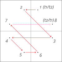
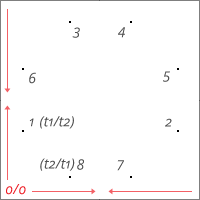
So, if c = 3, as in “dpy+3000”, the origin will be located at the lower left corner. What does this mean for our 8-dots display? Effectively, we’re plotting from the outside inwards, instead of inside-out, and the graph will “grow” from the corners:
Compare the emulation. (Sense switches may be operated either by the options menu at top right of the emulation or by holding the SHIFT-key and pressing the corresponding number key.)
(Screenshot of the program running in emulation.)
For a complete disassembly of “snowflake_sa-100.bin” see here.
Here we may also find a reason for there is so little known about the origin of the program, as the starlike display graphics seem to have been patched in rather late in the process, which may suggest that the name “Snowflake” was only later attached to a program that may have been known by another name while in development — and consequently may have been still known by this original name at the installation it originated at. (Hence, to risk a pun, nobody knew how to connect the dots.)
And this was it for “Snowflake SA-100” in particular, and for this walk trough the code of Snowflake in general. — Don’t hesitate to contact me in case of any corrections or for providing further information!
Norbert Landsteiner,
Vienna, 2019-01-10
Discuss/comment on Hacker News or (while it lasts) Google+.
P.S.: For more PDP-1 related software archeology, see my analysis of Spacewar!, the first digital video game.