A closer look at Marvin Minsky’s “Tri-Pos” display hack for the PDP-1.
Image: montage, photo of Minskytron at CHM by Joi Ito (CC 2.0).
→ I’ve read this already, take me to the playground.
Note:
This is an unfinished and unreleased article! Especially the introduction and most of the interpretation & contextual evaluation are missing. Still, the remaining may be interesting to some.
So, instead of an instruction, here are some quotes, which were meant to set up the theme:
With the software taken care of we could write real programs, which is to say toys. Bouncing Ball was successfully converted to PDP-1 use, but HAX, for some reason, was not. But no one really missed it, because we had a brand-new toy invented by Professor Marvin Minsky. The program displayed three dots which proceeded to “interact,” weaving various patterns on the scope face. As with HAX, the initializing constants were set in the console switches. Among the patterns were geometric displays, Lissajous-like figures, and “fireworks.” Minsky‘s program title was something like “Tri-Pos: Three-Position Display,” but from the beginning we never called it anything but The Minskytron. (“tron” was the In suffix of the early 1960s.)
“The Origin of Spacewar” by J.M. Graetz, Creative Computing, August 1981 (Volume 7, Number 8)
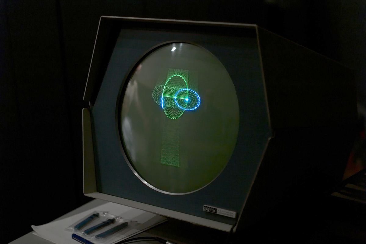
The Minskytron at CHM, photo by Joi Ito, 2007 (CC 2.0).
Marvin Minsky had written a little program that puts some dots on the display and ran them around, but it didn't do very much and you puttled on the switches looking for different starting values to get an interesting pattern, but most of them didn't work very well. So, it didn’t have, what we call now good play value.
Steve Russell at the Computer History Museum’s (CHM) “The Mouse that Roared: PDP 1 Celebration Event” (video)
Anyway, the PDP-1 arrived, and Marvin Minsky wrote the tripos demonstration, generally called the Minskytron, and there was the famous weekend where the mob of undergraduates transcribed the macro assembler from TX-0 to the PDP-1, because they didn't like FRAP. And then fairly quickly thereafter, they wrote DDT and connected up the macro symbols to DDT. So that was all sort of in place by the middle of the fall of 1961. And the combination of the Minskytron and having DDT with interactive debugging with symbols was very tempting. I don’t remember the exact order of things, but I’m pretty sure I started talking up a better demonstration program than the Minskytron (…)
Steve Russell, oral history interview by Al Kossow, rec. August 2008, CHM Catalog Number 102746453
Here is an elegant way to draw almost circles on a point-plotting display:
NEW X = OLD X − epsilon * OLD Y
NEW Y = OLD Y + epsilon * NEW(!) X
This makes a very round ellipse centered at the origin with its size determined by the initial point. epsilon determines the angular velocity of the circulating point, and slightly affects the eccentricity. If epsilon is a power of 2, then we don‘t even need multiplication, let alone square roots, sines, and cosines! The “circle” will be perfectly stable because the points soon become periodic.
The circle algorithm was invented by mistake when I tried to save one register in a display hack! Ben Gurley had an amazing display hack using only about six or seven instructions, and it was a great wonder. But it was basically line-oriented. It occurred to me that it would be exciting to have curves, and I was trying to get a curve display hack with minimal instructions.
“Item 149 (Minsky): Circle Algorithm” in HAKMEM, Programming Hacks. (MIT AI Memo 239, Feb. 29, 1972)
How to Draw a (Fast) Circle
Alan Kay, father of the WIMP GUI and many things, once gave in a talk a description of how a five year old, a 10 year old and a 15 year old would go about drawing a circle. (Given as an illustration of stages of development and dominant mental modes according to Jean Piaget and Jerome Bruner, which played an important role in the conception of GUIs.)
The five year old, being in a stage of bodily dominance, where the world is to be explored by doing, would come up with the solution of going a little and turning a little, going a little and turning a little, and so on, eventually achieving a perfect circle and inventing differential geometry on the way.
The ten year old, who is in a dominant visual mode and knows and loves a compass, knows that the points of a circle are on the compass line, all in the same distance from the origin, thus he would jump out from the center origin, mark a dot, jump back, turn a little, jump forth to the compass line, mark another dot, and so on. A somewhat more complex procedure, but eventually a circle, as well.
The fifteen year old, however, who has entered the symbolic stage, like a real grown-up, has learned about “x² + y² = r²”. Hence, there won’t be a circle at all.
So, how do we draw a circle?
And how can we do it fast? And, how can we fit the round — the circle — into the square — the grid units of our screen coordinates?
As we’re playing on a computer, the playful approach of the 5 year old may have some appeal, and, as we reduce the “a little” of the incremental steps to a minimum so that these are approaching zero, even Gottfried Wilhelm Leibniz will approve from a standpoint of differential calculus.
Still, how do these little steps correspond to our screen coordinates, and to what do these amount exactly, in order to give a circle?
Any versed mathematican will refer you to triginometry as the Rosetta stone of translations between the round and the square, since sine and cosine are just the projections of a rotated unit length onto the y and x axes, respectively. (Should this be confusing, refer to the figure below.) Thus, these give us the exact proportions of the offsets required, if we would desire to rotate a vector by a given angle θ.
x' = x × cos(θ) − y × sin(θ)
y' = x × sin(θ) + y × cos(θ)
However, sine and cosine are transcendental functions, lengthy and complex to calculate, maybe by a Taylor series, and computers aren’t neither fast nor good at it. (See here for how it’s done on the PDP-1.)
But, to our rescue and as any programmer in need of speed will tell you, the sine of an angle θ approaches θ for small angles, while its cosine approaches 1, providing a handy shortcut solution.
In order to appeal to your inner ten year old, here’s an illustration. We can easily see that for an angle of θ = 0 the sine will be zero and the cosine one, as the unit length extends along the x-axis. If we increase the angle by an infinitesimal amount, the sine will also increase by just an infinitesimal amount, just like the deviation of the cosine from the unit length of 1 will be just infinitesimal. And, since one infinitesimal epsilon is nearly as good as the other, the error will be infitesimal, as well.
But there is more to it. Computing the sine of θ in radians (where we divide the full turn of a circle into 2 × π units) is commonly done by a Taylor series like this:
So the first term is x, but what about the further terms? Now, looking just at the numerators and ignoring what’s below the line of these fractions, for a very small x, say, 0.0001 (1.0e-4), x3, the numerator in our first term, is 0.000000000001 (1.0e-12), and x5 is 0.00000000000000000001 (1.0e-20), which will probably just show as "0", if we’d try to enter it into a calculator. And these are just the numerators of our fractions! For all practical purpose and precision, these modifying terms after the first “x” are trending more and more towards zero, the smaller x (our angle θ in radians) becomes — leaving the bare, leading term x as a viable approximation of sin(x).
Even for an angle of 0.1 radians (~ 5,73°), the error is still rather small:
And, since “cos(θ) = sin(π/2 − θ)”, we may similarly, but with a bit greater error, substitute “cos(θ)” by “sin(π/2)” or 1, in order to avoid any computations at all. (Obviously, “1 − θ” may be an even better approximation, but this involves moving stuff between registers and performing an extra calculation, so 1 may be just good enough for a fast shortcut solution for a very small θ.)
As can be seen in the following table (this time appealing to your inner fifteen year old):
deg
rad
sin
cos
2.5°
0.04363323
0.04361939
0.99904822
2.0°
0.03490659
0.03489950
0.99939083
1.5°
0.02617994
0.02617695
0.99965732
1.0°
0.01745329
0.01745241
0.99984770
0.5°
0.00872665
0.00872654
0.99996192
0.4°
0.00698132
0.00698126
0.99997563
0.3°
0.00523599
0.00523596
0.99998629
0.2°
0.00349066
0.00349065
0.99999391
0.1°
0.00174533
0.00174533
0.99999848
0.0°
0.00000000
0.00000000
1.00000000
Sine and cosine for small angles, deviations from the approximations “sine(θ) = θ” and “cosine(θ) = 0.99999999” marked in red.
Hence, when using a very small amount — in common notation epsilon (ε) — for θ, we may substitute:
xn+1 = xn × cos(θ) − yn × sin(θ)
≈ xn × 1.0 − yn × ε = xn − yn × ε
yn+1 = xn × sin(θ) + yn × cos(θ)
≈ xn × ε + yn × 1.0
= xn × ε + yn = yn + xn × ε(terms swapped)
(Another way of looking at this is that the sine gives us the proportion of how far and in what direction to move along the y and x axes for any given turn in order to come up with a circle by incremental steps. As our steps and turns are suitably small and constant, we may substitute this by a small and constant factor epsilon.)
So we finally know how to draw a circle on the computer? — Sadly, no.
The reason for this is that our approximations are somewhat convincing, but not good enough for a full turn of a circle. There’s still an error involved, and, however small the error, it will accumulate over incremental steps as an outward drift (since our fast approximations are just a fraction too large) and the result will resemble more a spiral than a circle.
Which is, where Minsky’s lucky accident comes to the rescue: if we use the newly derived x for the mutation of y, the error will somehow self-correct!
Since this is best experienced to be believed (and to bring your inner five year old on board, as well), here’s a comparative animation of the two algorithms side by side (Minsky’s happy mistake on the right):
There’s still a small error (deviation from the ideal circle as shown in blue), but this is a pretty good circle!
(The result is actually a circle approximated by an ellipse rotated by 45°.)
As always, a smaller epsilon will mean smaller incremental steps and a better approximation. Let’s give it a try (epsilon = 1 / 32 ):
ε = 1/32
However, we’re not entirely there, yet. — Multiplications and divisions are another thing computers aren’t particularly good or fast at, especially, if there is no special hardware provision for this. But, coincidentally, shifting bits is something that is very essential to computers and they are really good at it. Shifting a binary number by a bit-position to the left amounts to a multiplication by 2 and, conversely, a shift to the right amounts to a division by 2.
Hence, by applying a number of right-shift operations (written “x >> n”) we arrive at divisions by the respective powers of two, which make for some nice epsilons:
x >> n  =  x / 2n  =>  ε = 1/2n

x >> 1  =  x / 21  =  x /   2
x >> 2  =  x / 22  =  x /   4
x >> 3  =  x / 23  =  x /   8
x >> 4  =  x / 24  =  x /  16
x >> 5  =  x / 25  =  x /  32
x >> 6  =  x / 26  =  x /  64
x >> 7  =  x / 27  =  x / 128
x >> 8  =  x / 28  =  x / 256
x >> 9  =  x / 29  =  x / 512
So, now we finally know how to draw a fast circle on a computer, thanks to Marvin Minsky, and it can be all done by fast integer operations!
XNEW = XOLD − ( YOLD >> n )
YNEW = YOLD + ( XNEW >> n )
Why this is so exactly is a bit mysterious, as pointed out by Rich Schroeppel in HAKMEM Item 150, in the style of a kōan (which were somewhat fashionable at MIT AI Lab):
“PROBLEM: Although the reason for the circle algorithm's stability is unclear, what is the number of distinct sets of radii? (Note: algorithm is invertible, so all points have predecessors.)”
Having thus tackled the arithmetic premise, we are essentially ready to dive into the program. But, before we have a closer look at the code, we’ll first have a glance at the machine it affects, in order to understand how it does it.
A Quick Introduction to the PDP-1
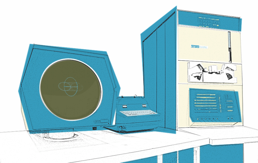
DEC PDP-1 (artsy)
The DEC PDP-1 (Digital Equipment Corporation’s “Programmed Data Processor – 1”) was introduced in 1959 after a quite short development phase of just three-and-a-half months, and first production protypes were delivered in 1960 with production units (PDP-1C) becoming available in 1961. Depending on its use, the PDP-1 may be categorized either as an early workstation (probably the very first one to be built in series) or as a small mainframe computer. It was the first commercial interactive realtime computer that came with a display (and optionally a light pen), bringing the kind of experimental computer technology developed at MIT to a broader market. (The US armed forces had already a go on this with the SAGE system. Allegedly — I struggle to find a source —, DEC’s motivation for entering “Phase 2” of its development plan and to build a computer was an anticipated request by the USAF for a missile interception control system — well, kind of a mini-SAGE in a box.) The PDP-1 came at a reasonable price, but — at US$ 120,000 in 1960 money — before computers became subject to enconomies of scale, this was still affordable only to institutions and corporations with a serious commitment to the nascent computer age. Still, the PDP-1 cost less than a single input/output channel for a contemporary IBM mainframe. The BRL Report from 1961 remarks,
The machine has an unusually high (>1) operations per second to initial cost ration[sic]. It is, thus, well suited to many real time control problems and is an excellent machine for interp[r]etive programming. Greater than 100,000 operations per second, flexible input-output, and powerful order code for a machine of this size.
(Ballistic Research Laboratories, A Third Survey of Domestic Electronic Digital Computing Systems, Report N0. 1115, Martin H. Weik, March 1961, p. 0765)
PDP-1s were used for simulation, experimental image recognition and speech input, a PDP-1 at LLNL even featured a mouse (an improved in-house design based on Engelbart’s original SRI design) by the mid-1960s before the mouse made an appearance in the “Mother of All Demos”, it saw early CAD applications, demoed timesharing, but it was also deployed for more humble mainframe tasks like telephone switching (branded as the ITT ADX 7300). Notably, a PDP-1 at BBN was used to develop and cross-compile the code for the first ARPANET gateways, the Interface Message Processor or IMP for short, and it was also the machine that inspired the conception of the very first digital video game, Spacewar!, at MIT. Quite a remarkable machine, which saw many notable applications and quite a number of firsts in software development and applications. And, according to Ed Fredkin, the PDP-1 even inspired the IBM RISC architecture developed by John Cocke, thus its architecture lived on in the IBM 801 and the IBM RS/6000.
While higher languages and timesharing systems became eventually available, the machine was originally thought to serve a single user at a time (the closest you could get to a personal computer by 1960), who would operate the machine “bare metal”, without any intermediate OS, instructing it directly in assembler code. Which is also, why we need to have a closer look at how this works.
Technicalities
Technically the PDP-1 was/is a 18-bit machine with an address bus of 12-bit, good for 4K of 18-bit words of core memory, which was also the standard complement. However, memory could be expanded to up to 64K by adding up to 15 further memory modules and applying bank switching. (Core memory was still prohibitively expensive and a module of 4096 18-bit words figured at US$ 30,000 in the 1963 price list.)
For signed numbers’ arithmetic the PDP-1 used one’s complement, which is simply all bits of a word flipped. While this is straight forward, it provided an extra value, namely negative zero (−0) with all bits set high (octal 0777777), which is why we eventually switched to two’s complement representation, where we add 1 to the negated number in order to skip this extra value.
The PDP-1 used a single-word instruction format, combining a 5-bit instruction code and the address (or operand) in a single word, separated by an extra bit in the middle. This extra bit, the i-bit or defer bit, provided indirect addressing for any instructions accessing memory and could modify some of the internal instructions, like reversing the condition for conditional skip instructions. (The PDP-1 used skips of the immediate next instruction, rather than branching to a distant address, leaving it to the programmer to decide what to do next.)
PDP-1 Instruction Format:


                      1 1 1 1 1 1 1 1
  0 1 2 3 4 5 6 7 8 9 0 1 2 3 4 5 6 7    bits*
┌──────┴───┬─┼─────┴─────┴─────┴─────┐
│  opcode  │i│   address / operand   │   instruction format
└──────────┴─┴───────────────────────┘

*) bits were numbered by DEC from left to right,
   starting at the most significant bit.
Instructions internal to the CPU completed in 5 microseconds (providing a speed of 200 KHz or 200 kilocycles, as it was then dubbed) and any memory access added another 5 microseconds to this. (As did any step of indirect addressing, of which there could be multiple, as the i-bit was evaluated at each memory access.) While this may not seem fast by modern standards, the versatile instruction set made up for it. For example, there is an “index and skip” instruction, which increments the contents of a given address and skips the next instruction (usually a jump), if the result was positive, providing the basic building block for a count-down loop, or there were quite powerful shift and rotate instructions supporting bit-shifts by up to 9 positions in a single CPU cycle.
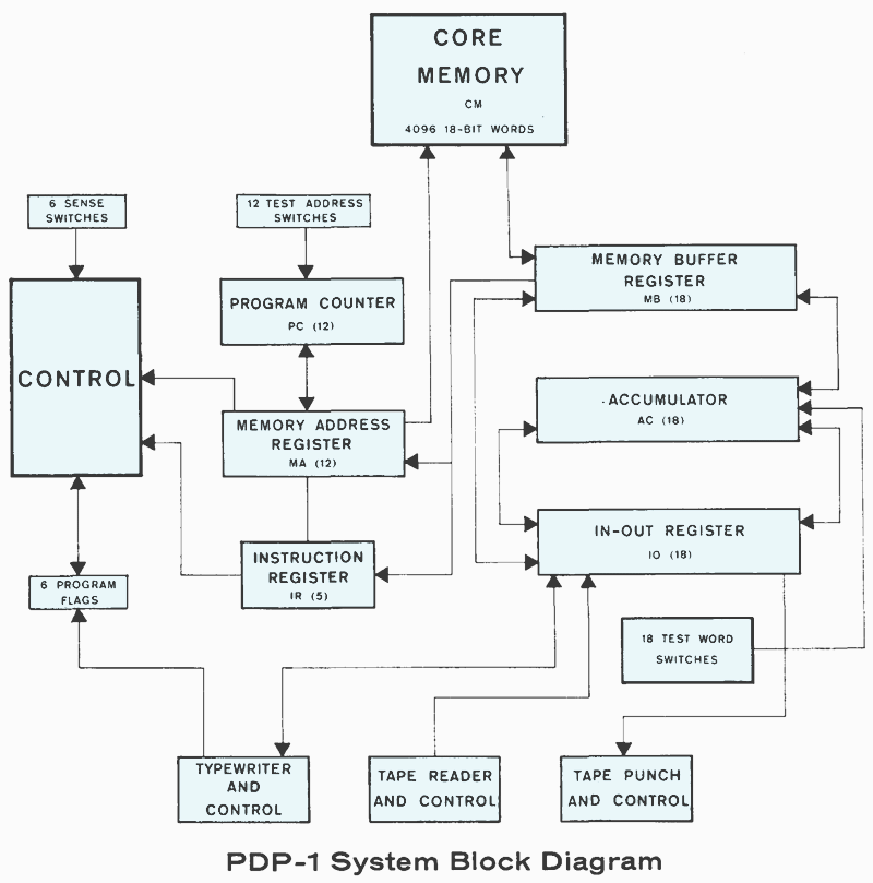
PDP-1 System Block Diagram Source: PDP-1 Manual, F-15B, DEC 1961, p.7 (edited; N.L.)
There are two 18-bit registers useful to the programmer, the accumulator (AC) and input-output register (IO). For some operations, like shift and rotate instructions, these may be combined into a single 36-bit register with the accumulator in the upper part. Almost all operations take their operands from memory, with the lower 12 bits specifying the address to look for. As the PDP-1 was designed before hardware support for higher languages became a thing, there are no index registers ands there is also no processor stack. What the PDP-1 has instead of a stack, are special instructions to deposit a value only in the address part or the instruction part of a memory word. This allows to modify instruction on-the-fly, not an unusual procedure at the time, e.g., a necessity for performing a return from a subroutine.
Something to take note of is that, before octet bytes took over, bits used to come in triples (notably 18 is 6 × 3). 3 bits at a time are quite easy to parse for humans and translate to octal digits ranging from 0 to 7.
011 …… 3
110 …… 6
010 …… 2
100 …… 4
111 …… 7
...
Hence, octal numbers were commonly used as the default number system in code and we'll stick to this further on, if not explicetly noted otherwise. E.g., the full 18 bits provide a range from 000000 to 777777 and the 12-bit addresses range from 0000 to 7777.
The Type 30 CRT Display
Since we're investigating a graphics program, it may be worth having a look at the display, as well. At that time, maintaining a bitmapped display was totally untinkable, both because of limitations of the memory technology available and for the horrendous costs that amount of core memory and supporting circuitry would have caused. So, X/Y displays was the way to go.
In its simplest form a X/Y display is just an oscilloscope: you apply suitable voltages for the x and y coordinates and activate a spot. Preferably, this supported digital inputs and mayby varying intensities of spot illumination. This is essentially, what the Type 30 display is. (In actuality, it is a bit more complex than this, it supported a light pen, incorporating cooling circuitry for the deflection in order to provide a sharp and stable picture and to prevent overshoot and undershoot, when moving the beam rapidly from one display location to another across the screen, and it even featured logic for asynchronous communications with the computer, so that the PDP-1 could progress on its tasks, while the display was going around its business.) This comes with both caveats and bonuses: On the one hand, as there is no display memory, this requires the programmer to take care of redrawing the screen and to keep the main loop as stable as possible for a flicker free display. On the other hand, as emphasized by Marvin Minsky, it was probably never that easy again to put a dot on the screen: just tell the display X and Y and forget about it. According to Minsky, computer graphics just went into decline with raster displays.
DEC Type 30 CRT Display Source: Precision CRT Display / Type 30E, F-15(30E), DEC 1963, p.1-2.
The Type 30 CRT display supports a technical resolution of 1024 × 1024 display locations (there are no pixels) and it does so at 8 possible intensities (spot brightnesses). However, as these locations slightly overlap, this provides — according to DEC — a visual resolution of 512 × 512 discernable display locations. You address the Type 30 by putting the X coordinate in the accumulator (AC) and the Y coordinate in the IO register and issuing a display instruction (which may include options like the intensity to be used). The display will take the top-most 10 bits and interpret them as a signed 10-bit integer, with the origin of this coordinate system in the center of its circular screen, the positive x-axis extending to the right and the positive y-axis pointing up.
Display coordinates of the DEC Type 30 display. −511 at the very left and very bottom. (0|0) is immediately right and above the center, (−0|−0) is immediately left and below the center origin. −0 is octal 01777 in 10-bit one’s complement.
For our graphics program, the important thing to take home is that we just issue display commands and forget about them (without any need to clear the display), but we should do so on a regular basis. Also, thanks to the display observing only the top 10 bits, this transforms anything related to display locations into fixed point numbers with a signed 10-bit integer part and 8 fractional digits.
The most remarkable feature of the Type 30, however, was its display tube: high resolution CRTs for RADAR scopes were readily available, and this is what the Type 30 used. Specifically, this one featured a P7 phosphor, a dual coating where one type of phosphor reacts in bright blue for just a short period, while a second, yellowish-green one provides a long sustain, which can remain visible — depending on the lighting conditions — for several seconds. This not only helps with image stability, it also puts an emphasis on any moving objects that will leave characteristic trails on the display. Arguably, this makes the Type 30 not only a X/Y display, but, by adding a temporal component, a 3-dimensional display, where any motion is reflected by the length of the trails and their respective gradient. Which is not only of aesthetic interest, but crucial for the animations of the Minskytron.
The Code
Marvin Minsky’s “Tri-Pos” display, commonly known as The Minskytron, varies the fast circle scheme, we’ve investigated above, in a decisive point: here, it’s not just the shifted respective other coordinate that modifies the x and y coordinates, but the shifted difference between this and respective coordinate of the next oscillator in the line that make the modifying term, thus chaining up and interconnecting 3 individual circle generators. Each of the generators will be modulated by the output of the next one in the line and will in turn propagate its new state to the previous one in the next iteration of the animation loop. Moreover, the Minskytron allows the operator to set up the amount of bit-shifts that are to be applied to each of these modifying terms, thus providing a rich variety of generated patterns by adding scaling and distortion to the individual generators.
We do not have the original source code as written by Marvin Minsky, but we do have the binary object code. Here, we’ll discuss it in disassembly with symbols and labels as used by Peter Samson, who disassembled and reassembled the propram as it is seen today at the CHM demos of the fully restored PDP-1. We do not know what assembler Minsky would have used, if this was FRAP (Fredkin’s “Free of Rules Assembler Program” fitting into the just 1K of memory of the first prototype) or MIT’s Macro (ported from the TX-0). We’re using Macro’s syntax (which doesn’t matter much, as the code doesn’t use any of the more specific assembler features and standard instruction names had been assigned by DEC), all numbers are octal.
So, here is what we know, in octal, instruction codes, and symbols:
Just kidding. Of course, we’re going through the code line by line, instruction by instruction, and we’ll probably start best at the very beginning.
500/
       lat
       rcl 9s
       rcl 9s

m1,    jsp gsh
       ...
The workings of an early assembler are not that mysterious: if there is anything on the very beginning of a line, followed by a comma, this defines a label (consisting of a letter, followed by up to two letters and/or digits), a symbol which may be used anywhere else as a stand-in for the address, where this was defined. Almost anything else in a line is just added up by the assembler, substituting symbols and instruction codes, which are just predefined symbols. There are a few exceptions to this rule, especially comments, which start with a slash (“/”, anything behind this will be ignored by the assembler) and some pragmatic rules instructing the assembler how to procede.
The very first line is such a pragmatic pseudo-instruction, telling the assembler the very address, at which to start generating its code In this case, it’s probably not the original start address, but what’s used by the CHM, otherwise, it’s not of further interest. Every program has to start somewhere, in this case at the (octal) address 500.
From the Beginning (Setup)
So, let’s have a go at it, for real:
       lat         / load test word into AC
       rcl 9s      / rotate AC and IO by 9 bits to the left
       rcl 9s      / rotate AC and IO by 9 bits to the left
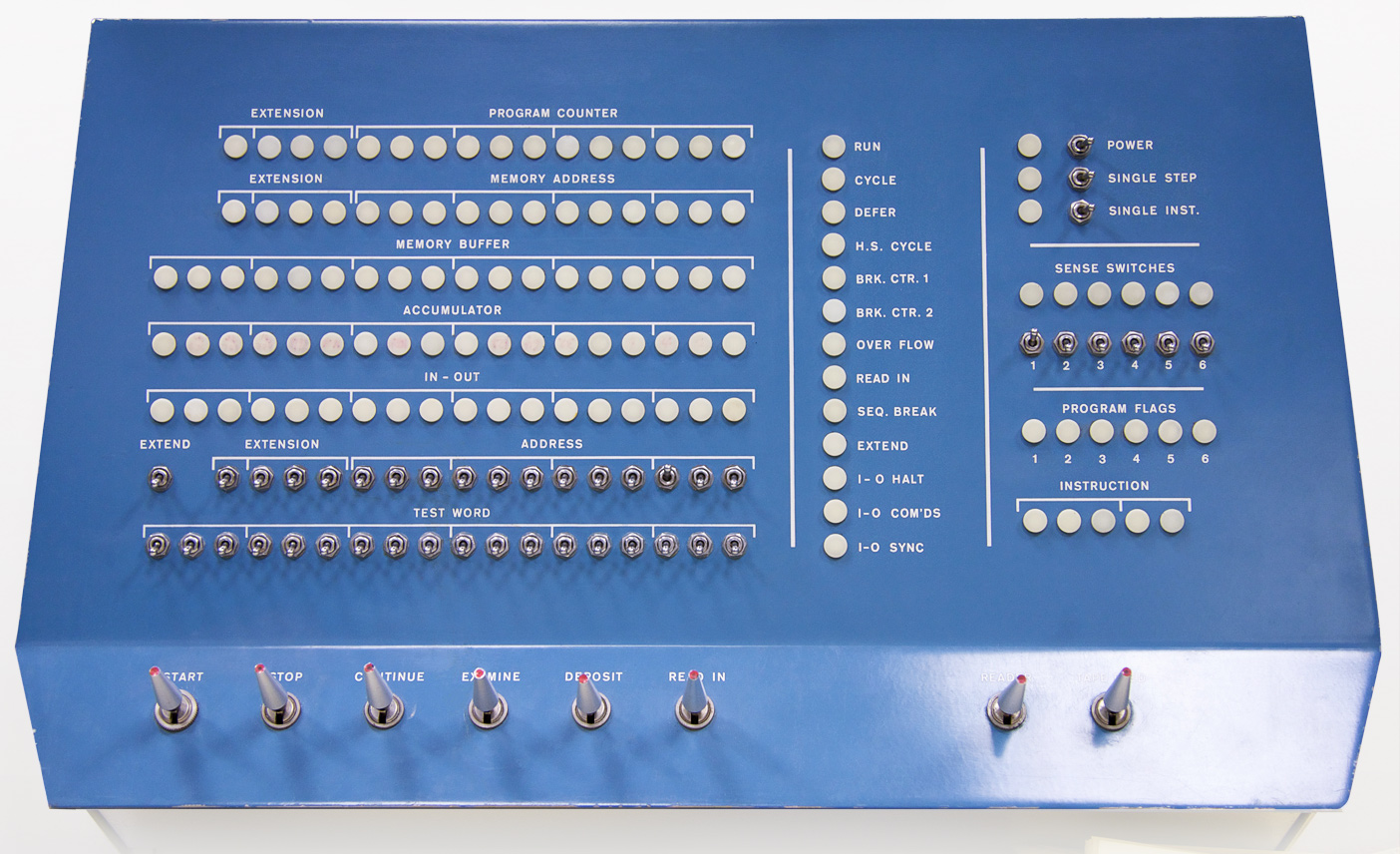
The first instruction “lat” (which probably stands for “load accumulator test word”) loads the Test Word into the accumulator. So, what is the Test Word? It’s an array of switches that allows us to assemble an 18-bit word on the control console of the PDP-1, which we may either deposit manually in memory or which may be read by the program thanks to this instruction. Here is what it looks like on the fancy, hexagonal console of the PDP-1, the last row of switches on the bottom left:
Mind how the bits are divided by the markings into groups of three, which will matter later. — Anyways, whatever is set up on those toggle switches (a switch in up position sets the respective bit to high, a switch in low position indicates a zero) will be transferred into the accumulator.
(We may also observe how the program will be started: we simply flip the power switch at the very top-right, and, assuming our program is already in the non-volatile core memory, we’ll enter address 500 in the row above the Test Word, by flipping the first and last switch in the third triple from the right to up and all others to low. Then we’ll start the program by deploying the Start switch at the very bottom-left.)
What follows are two “rcl 9s” instructions. We already mentioned that the PDP-1 can combine AC and IO into single 36-bit register for a few instruction, and this is one of them. This rotates the combined registers to the left: what is shifted out from AC will be shifted in into IO, and what is shifted out from AC will be shifted in into AC on the other side. We also mentioned how the PDP-1 rotates and shifts bits: by running in a micro-sequence over each of the lowest 9 bits and performing a shift or rotate for each bit set to high it encounters. The assembler has a handy set of predefined constants of this, named “1s” to “9s”, providing an appropriate bit-pattern for each of those shifts. The net result of this is that we rotate the two registers by an entire word-length of 18 bits. In other words, we just swapped the contents of AC and IO. (The PDP-1 had originally no dedicated instruction for this, only the later PDP-1D introduced a “swp” instruction.)
So we just read the number corresponding to the Test Word switches and transferred it into IO (as we may assume, for later use).
m1,    jsp gsh     / jump to subroutine at "gsh" (get shift)
       dac sh0     / deposit (store) contents of AC in location "sh0"
       jsp gsh
       dac sh1     / same for sh1
       jsp gsh
       dac sh2     / same for sh2
       jsp gsh
       dac sh3     / same for sh3
       jsp gsh
       dac sh4     / same for sh4
       jsp gsh
       dac sh5     / same for sh5
This seems to be a lot of the same. Having a closer look, it’s 6 times a “jsp gsh” instruction, followed by a “dac shn” instruction, where “n” is a number from 0 to 5.
“jsp” is a “jump to subprogram”, and what’s ever in AC after we return from this, is stored (“dac” is for “deposit accumulator“) at the addresses indicated by the “shn” labels. We find them at the bottom of the program:
sh0,   xx         / reserved for value sh0
sh1,   xx         / reserved for value sh1
sh2,   xx         / ...
sh3,   xx
sh4,   xx
sh5,   xx
(“xx” is a synonym for “halt“ and indicates that is a dummy-instruction just reserving space, rather than being meant for real. As this is not to be discerned by the binary object code, we have to attribute this to Peter Samson.)
So what’s at label “gsh”?
gsh, dap gsx / deposit return address in address part of loc "gsx"
cla / clear AC
rcl 3s / rotate AC and IO 3 bit positions to the left/ (highest 3 bits of IO now in AC)
add gsc / add conents of loc "gsc" to this/ (which is the address of label "gst")
dap .+1 / deposit result (AC + gst) in address part of next location
lac . / load contents of given address (as fixed-up before) into AC
gsx, jmp . / jump to return (address provided by instr. at "gsh")
gsc, gst / literal address of label "gst" (below)
gst, sar 1s / arithmetical shift right by 1 bit, ε = 1 ÷ 2
sar 2s / arithmetical shift right by 2 bits, ε = 1 ÷ 4
sar 3s / arithmetical shift right by 3 bits, ε = 1 ÷ 8
sar 4s / arithmetical shift right by 4 bits, ε = 1 ÷ 16
sar 5s / arithmetical shift right by 5 bits, ε = 1 ÷ 32
sar 6s / arithmetical shift right by 6 bits, ε = 1 ÷ 64
sar 7s / arithmetical shift right by 7 bits, ε = 1 ÷ 128
sar 8s / arithmetical shift right by 8 bits, ε = 1 ÷ 256
sar 9s / arithmetical shift right by 9 bits, ε = 1 ÷ 512 (not used)
This is probably the most complex bit of code of the Minskytron, but it is interesting to see how this code accomplishes its goals. What it it does, is basically extracting three bits (an octal digit at a time) out of IO and assembles the instruction code for an arithmetical shift to the right for the given number of bits + 1 on-the-fly. Which is also in AC, as the subroutine returns.
Let’s see how this is accomplished!
First, we somehow have to return to where we came from. However, the PDP-1 doesn’t have a processor stack to store the return address. What it does instead is simply putting the return address (the address we left at + 1) in AC. As a programmer, we’ve to deal with this. The means of dealing with it is the instruction “dap” (“deposit in address part”), which as already indicated by its name stores the value in AC in the given location, but only in the address part, leaving the highest 6 bits with the instruction code and the i-bit as-is. Thanks to this, we can fix up the “jmp” instruction at label “gsx”. Et voilà — here’s our return!
(We may observe some usual coding conventions (again, this is Peter Samson) at work: Related labels start with the same letter(s), an exit is usually marked by an “x” as the last letter, and an address that is to be fixed up by the program is usally indicated by a dot (“.”), which is actually the assembler notation for the current address.)
So, having taken care of the return address, we first clear the contents of AC (by the “cla” instruction) and are ready to go. Again, we encounter an “rcl” instruction, like we’ve seen it before, but this time, it’s only a left rotation by 3 bit positions. Since we’ve just cleared AC, and AC is in the high-value position of the combined AC-IO register, this will move the highest three bits in IO into AC. We have just extracted an octal number from what was in the Test Word switches! And we also prepared IO for the next extraction in the same step.
Next, “add gsc” adds to this whatever is in location “gsc”. What may this be? It’s actually the address of label “gst”, which serves as a base address of a list of 9 shift instructions with incremental numbers of shifts encoded. As this base address is added to the octal number extracted from the Test Word setting, we select the address of the instruction in the respective order.
The resulting address is now stored in the address part of the immediate next instruction by “dap .+1”. We’ve seen “dap” before, as we’ve seen the dot for the current address. As the assembler simply adds up what’s provided, this results in fixing up the address in the instruction that immediately follows. This is “lac .”, where the dot has been just replaced by the address we've just calculated before. As this is instruction is executed, we actually load the instruction code at the selected index from the table. And with this in AC, we happily jump to our return address.
So what’s this all about? As we can see, there’s a table of 9 shift instructions, which perform a right shift by an increasing number of bit positions (from 1s to 9s). Each of the triples neatly marked out on the PDP-1’s console represents an octal index into this table. As the first instruction is already a shift by 1 bit position, the respective shift instruction is this octal number + 1. We do this for each of the 6 octal digits of the Test Word and, as the subroutine ruturns, store the resulting instruction code in the loctions labeled “sh0” to “sh5”.
So, what’s special about this shift instructions? Now, an arithmetical right shift moves the contents of AC by the given number of shifts. However, instead of inserting what’s moved out on the other side, as with the rotate instruction, we simply drop the bits and repeat the sign-bit on the left side. By this, we get a division by the respective power of two — and it may not be the biggest spoiler ever, if we’d say that these are is the values of our epsilons, two of them for each of our three oscillators.
(Alternatively, we may think of a divison by 2n as a multiplication by a factor of 1/2n or, synonymously, by 2-n. This is really just a matter of nomenclature and we may use those synonymously.)
In other words — err, images —, what’s just happened is:
We just read the Test Word from the switches, extracted 6 octal digits, used them to look up instructions from a table, loaded them and stored them in 6 variables (sh0…sh5). These instructions correspond to right shifts or divisions by the given power of two + 1, therefore, a higher octal setup in the Test Word will mean a smaller value of epsilon.
Notably, the PDP-1 provides a shift-range of up to 9 bits per instruction, while there are just 8 octal digits. However, Minsky gives us the full list, but “sar 9s” will be never used. (As we've discussed before, the visual resolution of the Type 30 display is 512 × 512 or 8 bits and a sign-bit, so a shift to the right by 9 bit positions will never provide a visible result. Having to decide which one to skip, this one is a pretty obvious candidate.)
This highlight of self-modifying code is followed by a pretty triaval section:
m2,    lac xa0    / laod contents of "xa0" into AC
       dac xa     / deposit it in "xa"
       lac xb0
       dac xb     / xb ← xb0
       lac xc0
       dac xc     / xc ← xc0
       lac ya0
       dac ya     / ya ← ya0
       lac yb0
       dac yb     / yb ← yb0
       lac yc0
       dac yc     / yc ← yc0
We’re just copying some preset values into the memory locations that will be actually used by the program.
It may not be too preposterous to infer that these are three pairs starting coordinates (x and y, for a, b and c). However, what are these presets? We find them near the end of the program, just befor the locations that will be actually used.
Mind that, as far as the display is concerned, only the highest 10 bits are of interest. Which looks something like this, a slightly upright triangle with its base crossing through the center origin:
(0|0100)
b
a + c
(-040|0)(040|0)
(initial points in screen coordinates)
More precisely, it looks like this, if put these coordinates onto the display:
Tri-Pos!
Which is an image hard to unsee. I guess, there are those who have seen it and to whom it will be always the Tri-Pos, and those who have only experienced the fancy animation, to whom it will be the Minskytron.
Short Recap on the Setup Part
It may be worth to have another look at the initialization part, especially the subroutine “gsh”. The self-modifying code may seem enigmatic, even messy to modern eyes. Let’s recap why this would have been necessary, at all:
There is no processor stack and we have to somehow return to where we came from.
The PDP-1 uses a single-word instruction format, thus there are no separate arguments to instructions. Instruction codes and their operands share the same memory word.
There are no index registers to modify a given base address.
The “return problem“ is dealt with easyily enough by fixing up the address part of last jump instruction in the subroutine, and this has been somewhat an idiom on early computers, not just on the PDP-1. There would have been a way around this on the PDP-1, namely by indirect addressing. Every address can be made an indirect one by setting the i-bit. However, we would have to pay a penalty for this, namely an extra memory address to hold the return address and an extra execution cycle for the indirect memory lookup. Given that fixing up the address in place and executing it directly was the established way to do it, it just isn’t worth it.
The second problem solved by self-modification is the selection of an entry from a table. This is, essentially, quite easily accomplished: load the base address of the table, add the index to this, somehow load the value from this address. (We cannot simply assemble any of the “1s”…“9s” operands of the shift instruction, since this values aren’t linear, but actually represent numbers of bits set, from 001 to 777. Hence, these are stored in a table, together with the instruction code, ready to be used.) The problem arises with the “somehow load the value from this address“ part. Notably, on the PDP-1, like on most early computers, the operand of an instruction (with the exception of a few instructions that are entirely internal to the CPU) means, “the contents of this memory location.“ Therefore, we have to persuade the assembler to somehow store the base address of our table in a location, to which we may refer to in the addition. This is, where the construct
gsc, gst
comes into the picture: Here, the assembler just looks up the symbol “gst” (the base address of our table) and dumps it at location labeled “gsc”. Voilà, we can access our base address.
So, the code procedes to store the result of the base address added to the index in the load instruction immediately below and executes it in-place. Which is a simple solution to the problem, we’re confronted with. Again, we could have done the same using indirect addressing, but we would have paid a similar penalty. The only “luxurious” aspect here is the use of address “gsc”, we’ve just investigated. We just stated that an address always means the contents of this address on the PDP-1. However, there is an exception to this rule, namely the intrsuction “law n”, which loads a literal 12-bit constant n into the accumulator. Since addresses are just 12-bit, we could have used this to load the address immediately, without the round trip to memory. However, we want to add this value to the contents of the accumulator (resulting from the previous shift operation), not replace it. And, for addition, there’s no way around this.
There’s still something of note about this code, though. The way it addresses these problems isn’t what we’ll see below, when these shift instructions from the lookup table are used. So, is this actually Minsky’s code? We can’t be sure. The use of lookup tables was a common problem with common solutions, what we would call “patterns” today. Surely, Minsky wanted to have things just taken care of at this point, his central interest being playing around with the oscillation and display code. It may be a viable idea that he may have reused some code here and just inserted the shift-scheme for incrementially reading the octal values from the Test Word, which reside in the IO register at this point. We can’t be sure about this, but this is merely a pragmatic piece of code to setup the program. The important part here is the overall design, that we’re allowed to configure the Minskytron thanks to this setup code.
Curious Oscillations
So we’re finally arriving at the meat of the matter. Let’s have a look at the code for the first oscillator, which we call “A”, as the label ends in a distinctive “a”, just like the symbols for the coordinates associated to it.
m3a,   lac xa     / load x-coor into AC
       add xb     / add x-coor of osc. B to this
       xct sh0    / execute shift instruction stored in "sh0" (×ε)
       add ya     / add (old) y-coor to this
       dac ya     / store new y-coor
       sub yb     / subtract y-coor of osc. B from new y-coor
       xct sh1    / execute shift instruction stored in "sh1" (×ε)
       cma        / complement value in AC (AC = −AC)
       add xa     / add (old) x-coor
       dac xa     / store new x-coor
       lio ya     / load y-coor into IO
       dpy-i      / display a dot at (x: AC | y: IO)
So, what’s going here?
First we load the current value of the x-coordinate and at to this the x-coordinate of oscillator “B”, which is the next one in the line. We then execute the shift instruction stored in “sh0” by “xtc sh0”. (More on this a bit later.) Then we add the current value of the y-coordinate to this and store it as its new, updated value.
Unlike with later 12-bit mini computers, “dac” is not destructive on the PDP-1, so our new y-coordinate is still in the accumulator as we subtract the y-coordinate of oscillator "B" from this. Again, we execute a shift instruction (“sar sh1”) on the result. But then, unlike we’ve done before, we complement the value in AC (all bits flipped), resulting in a change of the sign, before we add the (old) x-coordinate to this and store this as the new, updated value.
With the updated x-coordinate already in AC, we load the y-coordinate into IO and use these as the x and y coordinates for our display instruction. While “dpy-i” may look a bit complex, it’s actually the most bare-bones display instruction. (Macro, in deviation from the DEC standard, expects you to want to use the “dpy” instruction with the i-bit, which is actually a modifier. Since Macro already encodes the i-bit and we do not want this to be set, we have to subtract it again to get the most basic form of the “dpy” instruction.)
So, what is this “cma” instruction all about?
Basically, if we complement a value, we flip all bits, what was a zero becomes a one and vice versa (same as XOR 777777.) Using one’s complement notation, this is the equivalent of changing the sign. By this, the following addition becomes a subtraction. This is even how the PDP-1 performs a subtraction internally, it first complements the value in AC, then performs an addition, and finally complements the result again. So, in theory,
a + −b = a − b
or in programmatical terms (1’s complement),
a + (b XOR 0o777777)  =  ((a XOR 0o777777) + b)  XOR 0o777777
                      =  a − b
At least, in theory. However, there’s always a difference between theory and praxis, and this applies even to a subject as platonic as mathematic. In our case, the addition “add” self-corrects for any result of minus zero by automatically adjusting it to plain zero, while the subtraction “sub” does not. (This is a deliberate design aspect of the PDP-1: “sub” actually skips the timing pulse in the micro-sequence, where this correction is performed for “add”.) There will be minor differences, which will add up and propagate. However, for the purpose of our explanation, we’ll stick to the platonic ideal and call this a subtraction (but keep in mind that Minsky is doing praxis here.)
but with the X and Y values of the next oscillator in line modulating the modifying term and using individual amounts of shifts (or values for epsilon) for each of the coordinates.
Returning for a moment to the curious “cma” instruction, we may observe that Minsky happily used a normal subtraction when it came to computing “YANEW − YB”. The net result of always using an addition for the outer term is that this operation will never yield minus zero for the new coordinate, as the addition auto-corrects.
Which raises the fairly interesting question, Was Minsky afraid of minus zero? To which I can only answer, I really don’t know. — And what a question, anyways!
There’s yet another point of interest here, namely how the shift operations are executed. Minsky uses here indirection, namely indirect execution. The instruction “xct” (execute) loads the contents of the given address directly into the instruction register of the PDP-1 and executes it. To modern eyey, this may be a horrible case of code-eval, but it is an elegant solution to the problem of applying varying shift instructions on a computer with single-word instructions.
But, there’s yet another aspect to this. We’ve seen before that the setup code avoided any indirection for a simple and fast approach. This could have been done here, as well. By simply inserting the shift instruction in-place, instead of storing them in separate locations, we could have achieved the same, but without the penalty for indirection, both in terms of space and CPU cycles. This would have been as simple as assigning the respective labels to those addresses:
(alternative form, not the original code)

m3a,   lac xa
       add xb
sh0,   .          / shift instruction stored here on setup
       add ya
       dac ya
       sub yb
sh1,   .          / shift instruction stored here on setup
       cma
       add xa
       dac xa
       lio ya
       dpy-i
However, Minsky (provided that our code is true to the original) decided to go with the more elegant and transparent solution using indirect execution. This may have been, because Minsky would have experimented first by simply altering constants directly by means of the toggle switches on the control console and added the interactive setup only later. We just don’t know. But the difference in the two approaches lets me think of the setup code and the actual display code as somewhat distinct entities.
From A to B and C (and Back Again)
This is followed by the code for oscillators “B” and “C”, where the coordinates of “C” are used to modulate “B” and those of “A” to modulate the ones of “C”, thus completing the circle, for which we jump back to oscillator “A”.
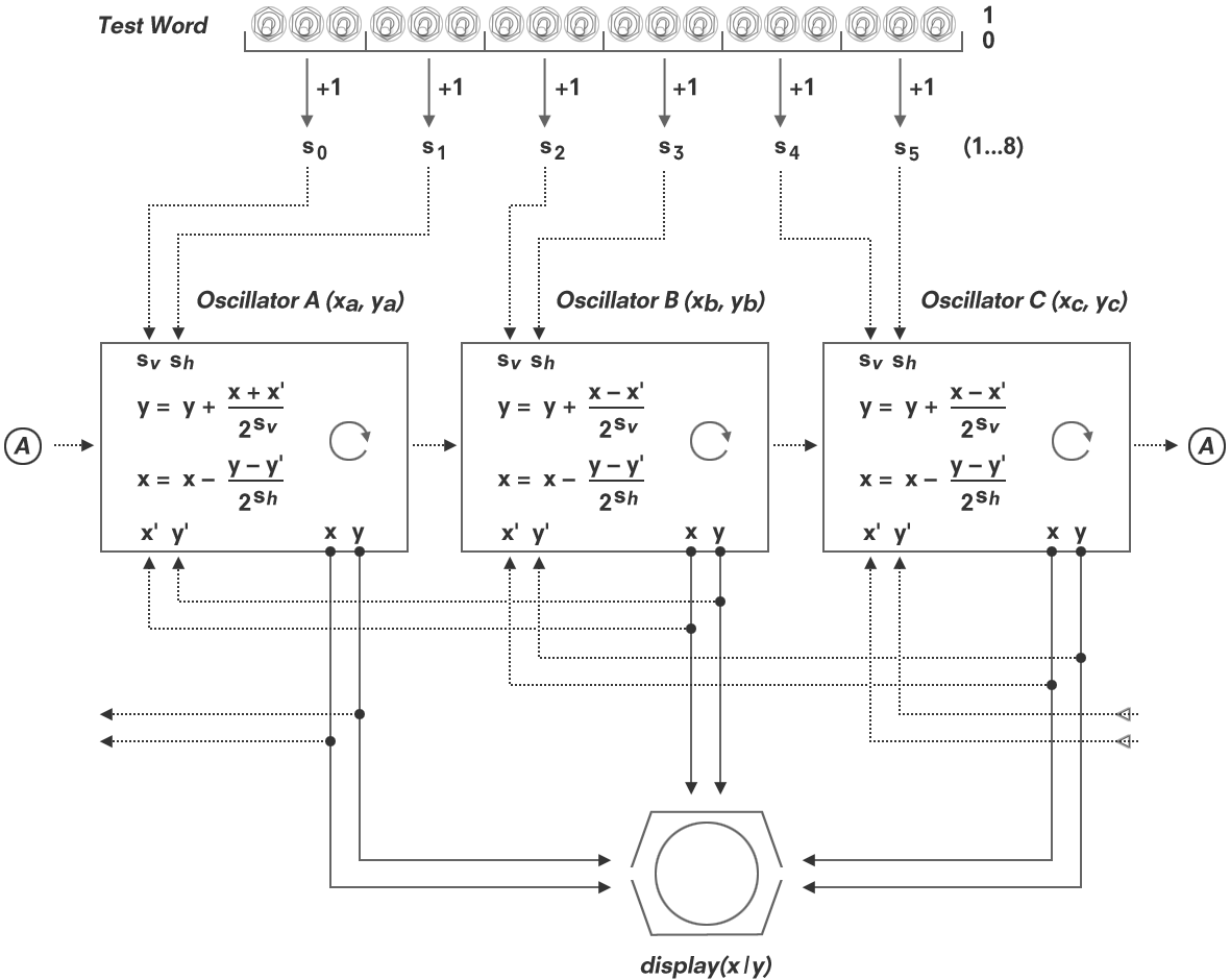
By this — believe it or not —, we’ve seen the entire code of the Minskytron. This finally allows us to paint the broader picture, namely
(For a difference, we’re here using simple integers instead of shifts for the setup and more general divisions by the repective power of two in the osillitators to emphasize that a higher input will mean an exponentially greater divisor for the modifying terms for each of the coordinates, and thus smaller vertical and horizontal increments.)
There are three oscillators — A, B and C —, which are really black boxes to the user. Each receives on setup an individual start position (not shown in the diagram) for x and y, and a set of scaling constants (sv, sh out of s0…s5), one for the vertical increment and one for the horizontal one.
Topologically, these oscillators are horizontally arranged and are visted in round-robin fashion. Each oscillator receives the current position (x', y') of the respective next oscillator in the line as another, variable input. Each osillator outputs its current position (x, y), which is plotted on the screen and serves as an input to the oscillator just before it in the line at the next iteration (or frame) of the main loop.
Internally, when called, these oscillators perform the fast circle algorithm, we already know. However, ignorring the modification by (x', y') for a moment, we may notice that the order of the operation has been swapped.
However, the order doesn't matter, it will be still a circle (or rather, a fat ellipse).
Another difference is that the procedure given in HAKMEM, Item 149, uses the same epsilon to produce the new x and y-coordinates, while the Minskytron configures individual parameters (sv, sh, as derived from the Test Word) for this at setup. Thus, we may scale (or distort) the circle by using asymetrical inputs.
But, before we dwell further into what these oscillators may actually do, we have to address the elephant in the room. As the observant reader may have noticed already, there’s a minor discrepancy or incongruence in those oscillators.
(You have not? — We have to talk. Really, I’m planting typographical hints, am preparing graphics, and you … you aren’t paying attention. So, here you are…)
While we’re genarally using the difference between the respective other coordinate of the oscillator and that of the next one as the base expression for our variations, the very first one, oscillator A, uses the sum to form this modifying term for the y-coordinate.
Let’s see what this effects to, when using a static oscillator (red, just a fast circle) to modulate another one (blue). On the left side the general form (as in B and C), on the right side what’s used for oscillator A:
This may look rather complex, but wait what happens, if we feed back the blue (modulated) oscillator into the red one, thus modulating them both in a feedback loop:
Two interconnected oscillators, each one modulating the other one. Left and right as above.
Now, the two symmetrical oscillators just form two circles around a common center, rotating at a 180° phase offset, while the two asymmetrical ones just head south in two almost parallel lines.
So what happens, when the two assymetrical oscillators break the bounds of our canvas? Here, we limit them to a toroidal space (where we enter on the opposite side, if we leave our limited space on either end; just what happens, when a binary number overflows). Accordingly, the lines reappear at the top, but, as the interconnected x and y-coordinates of the two oscillators get gradually out of sync, all kind of doodly figures start to appear. (If we did not happen to know that the image was the product of two interconnected oscillators, we may have a hard time figuring out how such complex and varying patterns may emerge from just two parallel lines.)
And, what may happen, if we dared to interconnect three of those oscillators, each one modulated by the next one in line? Well, that’s the Minskytron.
What’s important to note is that it is this asymmetry in the first oscillator, which adds progression and variation to the patterns generated by the oscillators. If we were to switch (spoiler: you may do so below) this first subtraction in the modifying term of the y-coordinate to an addition, as well, the pattern would stop to evolve and would become relatively stable. (Relatively, that is, as the oscillators are probably not perfectly in sync, as individual epsilons add distortion, hence the error of the fat elipse with regard to the ideal circle will gradually add up.) On the other hand, this asymmetry, which is driving the evolution of the pattern, is also its eventual demise, as the coordinates eventually overflow and all kind of weird, seemingly random patterns emerge, as the original, coordinated pattern breaks down.
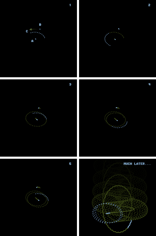
Pattern evolution of the Minskytron. (Test Word: 677721 = 7s/8s, 8s/8s, 3s/2s) Discrete brightnesses are an artifact of frame capture at 35fps, visual intensites are continuous on the original.
Let’s have a look at how the pattern evolves with the settings used by the CHM for their demos, Test Wort = 677721.
In #1, we’re about a dozen frames into the program. The dots drawn by A and B have hardly moved, at all (small wonder, as the increments are small with scaling factors of 2-7 and 2-8 for A, and 2-8 for both coordinates of B). Oscillator C, however, enjoys greater increments (at 2-3 and 2-2) and its dot has moved at constant speed, performing an arc in the counter-clockwise direction.
In #2, the arc described by C becomes descernible as a vertically squished circle (corresponding to its scaling by 1/8 and 1/4). Meanwhile, A and B have built up sufficient deviation from their initial coordinates to show some movement, as well. However, in accordance with their scaling settings, the increments are tiny and the overall Gestalt is hardly descernible.
In #3, directions of A and B become somewhat discernable. A is moving diagonally towards the bottom, by this dragging the entire configuration towards the bottom of the screen, causing C to fail to meet its starting point and to form a loop, describing a spiral instead. B is showing some modulation, as well, which may be best described as a slight “wiggle”.
In #4, oscillator A is clearly performing a generally linear movement, just what we observed in our experiment with two coupled oscillators. According to its scaling settings (2-7 and 2-8), the direction is almost diagonally towards the bottom right corner. It’s clearly oscillator A, which is dictating the motion of the entire configuration. While A is steadily performing its spiral, B is performing a series of “hops”.
In #5, the “hops” of B are lining up to a steady, irregular curve. But there’s also a noticeable deflection towards the center and this may be in fact a wiggely spiral. There’s also some barely recognizable deflection in the path of A, which starts to show some kind of bend, while C is just starting into its third circular movement.
Much later, we enjoy the pattern that has evolved from this: A is performing a broad, zig-zaggy waving motion in a general vertical direction, dragging the entire configuration accross the screen. The center of C is directly linked to A and the path described by its motion, while B is tied to A vertical motion only, performing a series of wiggly circles on it’s path accross the screen.
But what may happen, if we introduce the asymmetry of the addition on the x-coordinate, rather than on the y-cordinate? Well, have a look:
Minskytron with demo settings (Test Word: 677721), but the asymmetrical addition on the horizontal modifier of oscillator A.
We may still recognize the general pattern and its components, but this time, it’s moving horizontally, from right to left. Apparently, Minsky preferred the vertical evolution of the pattern.
We may try to reconfigure a horizontal setup by switching the shift parameters around so that it performs the same, exact motion as the standard version, but rotated by 90°. However, this will not work out. Why? Well, the triangle of the start locations is neither located at the center(rather, its base goes through the center origin ), nor is it an ideal, equally sided triangle (but slightly accute towards the top). As we rotate the setup but keep these positions, the triangle won’t be located at the central axis anymore. These locations do matter.
And what about the spread, the relative distance of these start loactions? If we were to spread them further apart (spoiler you may actually do so below), the pattern generated will be generally look the same, but there will be fewer iterations, until the coordinates overflow and the pattern breaks down. Overall, Minsky picked some nice and practical positions; not too far from one another, but far enough to produce a visibly discernible pattern right from the beginning.
Play Time
Time to do some praxis ourselves and to investigate and experiment!
Below, you find a reconstruction of the Minskytron, faithfilly emulating arithmetic operations, display and runtime of the PDP-1. However, there are also a few additions so that we can put some of our theoretical assumptions to a test.
Features
Pop-up menus may provide a more convinient and accessible way to select input parameters than groups of toggle switches, so we'll use these. (The original code selects values from a table by an index read from the input elements. This is exactly what the HTML select element does, in JavaScript terms, “selectedValue = SelectElement.options[SelectElement.selectedIndex].value”.) As we’re at it, we may also include the value “9s”, which had been included in the table by Minsky, but isn’t selectable in the original program.
We’ll include an option to define the initial spread of the three dots that produce the animation, so that we may explore the effect this has on the patterns generated. (This won’t be included for small screens, but you’re not missing much. As we increase the initial values, we’re scaling up the pattern produced and are thus shorting the time to it’s eventual break down.)
You may toggle the plotting of the individual oscillators on and off by clicking the respective plot symbols in the schematic provided along the emulated display, so you may explore which osillator generates which part of the pattern. (Unlike the controls mentioned previously, which only configure settings for the next run, you may do so anytime.)
Most importantly, you may click the operator icons in the schematic to flip them from addition (+) to subtraction (−) and vice versa.
Finally, we may want to verify that it is actually the limited 18-bit precision of the PDP-1, which causes the eventual break down of the patterns. Now, DEC originally planned a 24-bit version of the PDP-1 and reserved the name “PDP-2” for this. While the PDP-2 was never built as such, we can explore what it may have been like here. This is what the precision controls, found below the display area, are for. But how to procede with the display coordinates? Should we leave them as-is, starting at the 17th bit (counting from the LSB), thus preserving the display sale, or should we move it to the top of the word-size, as it is on the PDP-1? Why not do both? So there are options to move the bit range used for the display coordinates in steps of 3-bits, from the original position up to the top of a 24-bit word. This allows us to peek into a varying “window” in the total numbver space of the 24-bit precision at various scales and also decouples the display space from the number space of the underlying arithmetics, which may be interesting.
(You can use the form elements for this, but you may also just click respective elements on the precision/word-size display next to them.)
It should be mentioned that the emulation is best experienced on a larger display, which allows us to present the emulated in graphics in a round scope, which is quite important for the aesthetics of the Minskytron. Otherwise, we’ll fall back to displaying just the bare, square display area to make the best of the space available.
Default settings are those used by the CHM for their demos of the fully restored PDP-1.
So, well, here you are… enjoy!
A Minskytron Playground
Oscillator A
Oscillator B
Oscillator C
bits24 18
DISPLAY COORS
Precision:
Minskytron / Tri-Pos emulation (best experience on a large display). Select setup values and click “Start”. Click operator symbols and plot icons in the schematic to explore operations. (Mind that shift settings are +1 as compared to the original Test Word settings and include an extra option for "9s".)
Some Observations
A Modal Number Space
−
0
+
coor
value
octal
bits
localoct
localdec
x
0
0000
0000
0000
+0
y
0
0000
0000
0000
+0
Rant (UX)
Should you, dear reader, see the above range inputs (sliders) with an accent colored part extending from the left side (the so-called range-progress pseudo-element), this is a great example for where HTML goes downhill. Nothing in the definition of a range input suggests the idea that the value chosen by the user means the top of a range extending from the absolute minimum selected by the author. (Rather, it’s an arbitrary value chosen by the user from a range as defined by the author by an available minimum and maximum. In other words: the range is not what the user selects, but the section of the total from which the user picks a descrete value.) There is no need to add any such interpretation on the part of the browser, without any options for defining the meaning of the extent (e.g., as a deviation from the chosen preset value, which may make at least some sense in this case), if any, or to disable this behavior at all. As it is (or, more precisely, as it has now become), there’s only the option to confront users with an unfamiliar custom element, depriving them from their known and familiar interface, or to live with a nonsensical interpretation of a value, which isn’t called for by any means. But, yay, it’s colorful, we just made your website better! So, well, the number ‘4’ represents a range extending from ‘-1792’ (octal 04377 in 12-bit one’s complement) or 1796 units in total, which may come to a surprise to anyone slightly familiar with number theory. *sigh* — Great UX, folks!
P.S.: Should you, dear browser vendor, want to stick with this nonsense, please consider adding a CSS property ‘progress-origin’ with options like ‘min-value’, ‘max-value’, ‘preset-value’, a numeric value inside the given range, and — most importantly — ‘none’.
BTW, this is — apparently — what the quantity 75,000,000 looks like as a range.
(Image source gracefully redacted. Are you sure, you want to play in that league?)
Finally, should this be really the way to go, why shame users who want to select a lower value into higher values by sanctioning them by a less colorful presentation? Shouldn’t the range track adapt to a triangular shape with the acute angle pointing towards the maximum to assure a constant amount of colored area for a truly inclusive GUI? /s
The Minskytron in Context
But how does The Minskytron relate to Minsky’s other work?
Nowadays, Minsky may be better known for his critique of the Perceptron (or PDP, as in “parallel distributed processing”), especially regarding its limitations of modelling exclusive-or (XOR) functions. (Compare: “Perceptrons: an introduction to computational geometry” by Marvin Minsky and Seymour Papert, MIT Press, Cambridge, MA, 1969. [archive.org] According to Marvin Minsky, “It would seem that Perceptrons has much the same role as The Necronomicon — that is, often cited but never read.”)
This may overshadow the fact that Marvin Minsky was actually pioneering practical work, then still in hardware, and theoretical work on neural networks over the 1950s, starting with SNARC (Stochastic Neural Analog Reinforcement Calculator), built 1952 in Harvard from 3.000 vacuum tubes and a few parts from a B-52 bomber. Notably, SNARC, commonly considered as the first connectionist neural network learning machine, predates the publication of Frank Rosenblatt’s Perceptron (Rosenblatt, Frank, “The Perceptron: A Perceiving and Recognizing Automaton (Project PARA)”, Cornell Aeronautical Laboratory, Inc., Buffalo, NY, 1957. [PDF]) by several years. So, if anybody knew anything about neural networks and their implications for artificial intelligence (AI) by 1960, it was Marvin Minksy.
Compare:
“A Neural-Analogue Calculator Based upon a Probability Model of Reinforcement”, Harvard University Psychological Laboratories, Cambridge, MA, January 8, 1952; “Neural Nets and the Brain Model Problem”, Princeton Ph.D dissertation, 1954
“Some Methods of Heuristic Programming and Artificial Intelligence,“ Proceedings Symposium on Mechanization of Thought Processes, vol 1., Natl. Physical Lab., Teddington, UK, 1959
“Learning in random nets”, Marvin Minsky and Oliver G. Selfridge, Fourth London Symposium on Information Theory, Butterworth, Ltd., London, 1961.)
In 1960, just around the time the “Minskytron” was conceived, Marvin Minsky wrote the paper “Steps Toward Artificial Intelligence” [HTML, PDF] (published in Proceedings of the IRE, Volume: 49, Issue: 1, Jan. 1961), a general overview of the field, the advancements made, and the general state of affairs, where we find the following sections on the ‘hill-climbing’ approach (nowadays better known as ‘gradient descent’ as it is now about minimizing an error, rather than maximizing the output):
(If intimidated by the Greek letters λ (lambda), δ (delta) or μ (mu), feel free to read “x”, “d” and “m”, respectively.)
B. Hill-Climbing
Suppose that we are given a black-box machine with inputs λ1, . . ., λn and an output E(λ1, . . ., λn). We wish to maximize E by adjusting the input values. But we are not given any mathematical description of the function E; hence, we cannot use differentiation or related methods. The obvious approach is to explore locally about a point, finding the direction of steepest ascent. One moves a certain distance in that direction and repeats the process until improvement ceases. If the hill is smooth, this may be done, approximately, by estimating the gradient component δE/δλi separately for each coordinate λi. There are more sophisticated approaches (one may use noise added to each variable, and correlate the output with each input, see Fig. 1), but this is the general idea. It is a fundamental technique, and we see it always in the background of far more complex systems. Heuristically, its great virtue is this: the sampling effort (for determining the direction of the gradient) grows, in a sense, only linearly with the number of parameters. So if we can solve, by such a method, a certain kind of problem involving many parameters, then the addition of more parameters of the same kind ought not to cause an inordinate increase in difficulty. We are particularly interested in problem-solving methods that can be so extended to more problems that are difficult. Alas, most interesting systems, which involve combinational operations usually, grow exponentially more difficult as we add variables.
A great variety of hill-climbing systems have been studied under the names of “adaptive” or “self-optimizinig” servomechanisms.
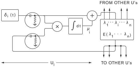
Fig. 1 — “Multiple simultaneous optimizers” search for a (local) maximum value of some function E(λ1, …, λn) of several parameters. Each unit Ui independently “jitters” its parameter λ1, perhaps randomly, by adding a variation δi(t) to a current mean value μi. The changes in the quantities λi and E are correlated, and the result is used to slowly change μi. The filters are to remove DC components. This technique, a form of coherent detection, usually has an advantage over methods dealing separately and sequentially with each parameter. (Cf. the discussion of “informative feedback” in Wiener [11], p. 133 ff.)
C. Troubles with Hill-Climbing
Obviously, the gradient-following hill-climber would be trapped if it should reach a local peak which is not a true or satisfactory optimum. It must then be forced to try larger steps or changes.
It is often supposed that this false-peak problem is the chief obstacle to machine learning by this method. This certainly can be troublesome. But for really difficult problems, it seems to us that usually the more fundamental problem lies in finding any significant peak at all. Unfortunately the known E functions for difficult problems often exhibit what we have called [7] the “Mesa Phenomenon” in which a small change in a parameter usually leads to either no change in performance or to a large change in performance. The space is thus composed primarily of flat regions or “mesas.” Any tendency of the trial generator to make small steps then results in much aimless wandering without compensating information gains. A profitable search in such a space requires steps so large that hill-climbing is essentially ruled out. The problem-solver must find other methods; hill-climbing might still be feasible with a different heuristic connection.
Certainly, in human intellectual behavior we rarely solve a tricky problem by a steady climb toward success. I doubt that any one simple mechanism, e.g., hill-climbing, will provide the means to build an efficient and general problem-solving machine. Probably, an intelligent machine will require a variety of different mechanisms. These will be arranged in hierarchies, and in even more complex, perhaps recursive structures. And perhaps what amounts to straightforward hill-climbing on one level may sometimes appear (on a lower level) as the sudden jumps of “insight.”
[7]M. L. Minsky and O. G. Selfridge, “Learning in random nets,“ in: Fourth London Symposium on Information Theory, C. Cherry, Ed.
[11]N. Wiener, “Cybernetics,” John Wiley and Sons, Inc., New York, N. Y.; 1948.
Now, there are some striking similarities. The horizontal topology of the Minskytron with its interconnected oscillators reminds very much of the horizontally interconnected optimizers given in Fig. 1, which are oscillators, as well. — May it be that the Minskytron isn’t so much a toy, but an experiment to exhibit human hill-climbing bahavior?
Indeed, the Minskytron provides the rare case where “human intellectual behavior (…) solve(s) a tricky problem by a steady climb toward success”, which is an exploration of the problem space provided by the Minskytron in the search of an aesthetically pleasing pattern. So, is the Minskytron a layer of optimizers, acting in reverse, in order to produce a problem space that is to be explored and solved by human hill-climbing strategies?
There are certainly “mesas” (e.g., around the standard setup used by the CHM), where tiny steps in any direction won’t have much of an effect on the animation, but then we fall of the cliff by just another step — there are also valleys, where find just snow or apparent visual noise — and the Minskytron is certainly a “black-box machine”, which achieves by its 6 inputs parameters (the shift factors) and 6 hidden variables (the coordinates) a sufficient level of complexity to be regarded as an “interesting system”.
It would have been a rare case of irony — or maybe “snow blindness” from too much exposure to similar experiments — had Minsky missed the similarities between his earlier work on neural networks and what he just had described in his paper on the one hand and his Tri-Pos arrengement on the other one, for this to be merely a coincidence. In the light of this, we even may not be too sure, whether we are meant to know that the Test Word is actually a compositum of 6 input parameters, or if it is rather meant to be regarded as just a row of arbitrary switch positions, as this will have certainly an impact on our search strategies.
If the Minskytron is indeed a riddle and not so much a toy, it poses some interesting questions:
There may not be an error function at all to minimize on, so that we have to employ a strategy of maximizing the output.
However, it may not be that clear, what maximizing actually means, what determines success. We may favor stability (that is, constraining the internal variable as best as we can to the bounds of the internal number space), aesthetic interest and variety, symmetry, motion, etc. We may even favor a setting, which will provide an interesting and somewhat coherent pattern after the break-down of the initial pattern, thus searching for (limited) stability in instability. Our goals may even vary, while we continue to explore the problem space.
Similarly, it may not be that obvious what error or failure may mean: what may be indiscriminate noise to one probant may be still a regognizable pattern in meta space to another person who has some understanding of the implication of a modular number space.
Is there even a curve to fit?
Is there even a problem? Certainly, there’s enough to give us a goal and to bind our interest, at least for some period of time.
What does “solving a problem” or “avoiding error” mean, if there are no clear definition of solution or failure, but still a viable interest in exploring the configuration in order to find a result?
Is there a classification or taxonomy of “viable” results? Is there a hierarchy to them? (Can we even quantatize “success”?) If so, is there a hierarchy of error?
If there is such a classification, is this ‘just’ an aesthetical one? Is there structure?
In Wittgenstein’s terms: Is there anything to speak about?
Certainly, there is something to be shown (e.g., at the CHM demos). — What is shown by the Minskytron?
Finally (still in Wittgenstein’s terms), is what is shown and what cannot be said, still subject to ML? (Are there similar problems?)
If the Minskytron was indeed a riddle or a test arrangement challenging human hill-climbing strategies, this may explain the inherent frustration with the Minskytron as an entertainment device, as expressed by the fathers of Spacewar!, who proceeded to invent video games in their search for a more capturing, “pleasurable” and “involving” entertainment in a “consistent framework”. (That’s hill-climbing! ;-) )
(I have to stress that I do not know anything about the background of the Minskytron, or Tri-Pos display, as I haven’t been able to determine anything about the circumstances under which it emerged or to even attribute a date or a place or institution to this. Please mind that this is — while it may be an intriguing conjecture — pure speculation and not founded in any any hard evidence.)
Another Perspective
So far we described (probably somewhat period adequately) the Minskytron in terms of oscillators / vibrators, modulation, and feedback loops. But there is also another, maybe more modern perspective, emphasizing how signals propagate through the network that‘s formed by the individual elements elements.
The Minskytron as a recurrent neural network (RNN) plotting X and Y over time. Layers X and Y are dynamic, while Wx(a…c) and Wy(a…c) are static, but configurable.
Final Considerations and Another Minskytron
So our investigations of the Minskytron as a visual toy, our efforts to make its inner workings transparent, may have been mistaken altogether. Still, it would have required these insights to understand what may be actually shown by its arrangement, what is posed as a more general question, should it have been meant as a challenge to problem solving in a much more general way. But, maybe, it was just Marvin Minsky playfully reversing the experimental setups he was investigating at this time. We really don’t know.
Anyways, whatever the Minskytron was meant to be, to us, nowadys, it’s a digital toy, a visual synthesizer. As, such, I think, our own test arrangement shows that it benefits in variety from a facility to flip the operators from addition to subtraction and vice versa, as this adds new classes (or sets) to the patterns it may generate. By sheer coincidence, there is a set of yet unused interactive controls on the operator’s panel of the PDP-1, and by yet another amazing coincidence (or rather, thanks to the consistency of the underlaying design principles of the PDP-1), there are 6 of them, exactly what we need!
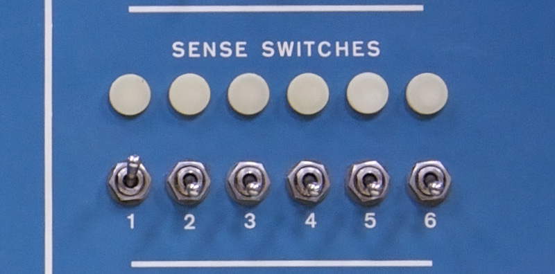
These are the ‘sense switches’ (so called, because David Byrne will show up and tell you to stop making sense, if you’re caught playing too much with them — or, maybe, just because the state of these switches can be sensed by the machine — are you still paying attention? ;-)), and they even have nice lights to indicate, whether they are on or off. While an additional set of operator’s controls wouldn’t have made any sense (or would have been even counter-productive) for the Minskytron as a testing ground for human hill-climbing behavior, we should really make use of them.
We’ll assign them in the same order already used for the Test Word: switch 1, the very left most of the switches, will select the operation for the vertical modifier of oscillator A, the same one, sh0 operates on, and so on. A switch in down position (off) will mean to apply a subtraction as the default operation and up (on) will mean addition.
Minskytron II
As we we’ll see, we can read the switches and configure the program at setup without affecting the runtime part of the program at all. We’ll call the resulting program the “Minskytron II”, because, well, it’s the Minskytron, too. (Admittedly, this isn’t the best joke ever.)
While “dap”s (deposit AC in address part) are all over the place in PDP-1 code, I’ve rarely seen its counterpart “dip” (deposit AC in instruction part). So this may be an opportunity to give it some exposure, since assining the operation to a given operand is exactly what we intend to do. (As a recap, “dip” only affects the instruction part or the 6 most significant bits of an instruction word, while the address part or operand remains as-is.)
For reading (or ‘sensing’) the state of a switch, the PDP-1 provides the conditional instruction “szs” (skip on zero sense switch #n), which skips the instruction immediately next in memory, if the given sense switch is not set (off). (As this is a member of a micro-coded instruction group, the number of the switch is encoded in the second lowest octal digit, bits 6—4 in modern notation.)
To make appropriate use of these instructions, we’ll first load the instruction code of the subtraction (“sub”) into AC, then check the sense switch and skip the next instruction, if the switch is off. Should the switch be on, however, we’ll execute the next instruction, which loads the instruction code for the addition (“add”). Then, we’ll deposit whatever instruction code is now in AC (sub or add) in the instruction part of that memory location in the main loop which adds or subtracts the coordinate from the next oscillator, thus modifying the operations of the program.
So, in order to ‘sense’ switch #1 and to configure the program, all we have to do is inserting the following code, just after the setup of the shift factors has completed and before the start of the main loop:
/ just after setup complete
mss, lac ops / load instruction code for subtraction
szs 10 / is sense switch #1 set?
lac opa / yes: load instruction code for addition
dip m3a+1 / insert it in instruction part at the location just
/ after label 'ma3' (sub/add xb)(...)
/ at the end of the program
opa, add / inserts the instruction code for 'add'
ops, sub / inserts the instruction code for 'sub'
(Mind that we cannot use “law”, because this loads just a 12-bit value and the instruction code is exactly out of range. So we have to add yet another table at the end to read those instruction codes as constants.)
Repeating this pattern for each of the 6 switches and operators provides the entire modification. A modification, which leaves the main loop totally uneffected in terms of runtime performance:
minskytron ii
/ based on dpys5, pdp-1 display hacks(...)/ insert just after setup code
mss, lac ops
szs 10 / m3a: (add xb), if sense switch 1 set, else (sub xb)
lac opa
dip m3a+1
szs 20 / m3a: (add yb), if sense switch 2 set, else (sub yb)
lac opa
dip m3a+5
lac ops
szs 30 / m3b: (add xc), if sense switch 3 set, else (sub xc)
lac opa
dip m3b+1
lac ops
szs 40 / m3b: (add yc), if sense switch 4 set, else (sub yc)
lac opa
dip m3b+5
lac ops
szs 50 / m3c: (add xa), if sense switch 5 set, else (sub xa)
lac opa
dip m3c+1
lac ops
szs 60 / m3c: (add ya), if sense switch 6 set, else (sub ya)
lac opa
dip m3c+5
m3a, (...) / main loop/ to be added at the end of the program
opa, add
ops, sub
As the only noticable difference to the traditional program we’ll now have to put sense switch #1 in on position and all others to off for usual operations.
If you happen to have an operational PDP-1 around and want to play along “at home”, you can download the source code here and the resulting binary (or “octal”) here, or the entire package as a ZIP-archive: here.
(to be accompanied by a merry melody) — That’s all, folks! —
As always, any comments and/or corrections are welcome.